16. CHAPTER 16. CHECKING THE MODEL AND DATA

SET UP

library(foreign) # to open stata.dta files
library(psych) # for better sammary of descriptive statistics
library(repr) # to combine graphs with adjustable plot dimensions
options(repr.plot.width = 12, repr.plot.height = 6) # Plot dimensions (in inches)
options(width = 150) # To increase character width of printed output

Load Libraries

Show code cell source Hide code cell source

pkgs <- c("car", "jtools", "sandwich","huxtable","dplyr","olsrr")
invisible(lapply(pkgs, function(pkg) suppressPackageStartupMessages(library(pkg, character.only = TRUE))))

16.1. 16.1 MULTICOLLINEARITY

df = read.dta(file = "Dataset/AED_EARNINGS_COMPLETE.DTA")
attach(df)
print((describe(df)))

              vars   n     mean       sd   median  trimmed      mad      min       max     range  skew kurtosis      se
earnings         1 872 56368.69 51516.05 44200.00 47580.66 24907.68  4000.00 504000.00 500000.00  4.17    25.48 1744.55
lnearnings       2 872    10.69     0.68    10.70    10.69     0.57     8.29     13.13      4.84  0.10     1.01    0.02
dearnings        3 872     0.16     0.37     0.00     0.08     0.00     0.00      1.00      1.00  1.81     1.28    0.01
gender           4 872     0.43     0.50     0.00     0.42     0.00     0.00      1.00      1.00  0.27    -1.93    0.02
age              5 872    43.31    10.68    44.00    43.22    13.34    25.00     65.00     40.00  0.04    -1.03    0.36
lnage            6 872     3.74     0.26     3.78     3.75     0.30     3.22      4.17      0.96 -0.33    -0.93    0.01
agesq            7 872  1989.67   935.69  1936.00  1935.44  1054.13   625.00   4225.00   3600.00  0.39    -0.83   31.69
education        8 872    13.85     2.88    13.00    13.87     1.48     0.00     20.00     20.00 -1.04     4.67    0.10
educsquared      9 872   200.22    73.91   169.00   195.67    40.03     0.00    400.00    400.00  0.39     0.00    2.50
agebyeduc       10 872   598.82   193.69   588.00   593.70   187.55     0.00   1260.00   1260.00  0.14     0.54    6.56
genderbyage     11 872    19.04    22.87     0.00    16.59     0.00     0.00     65.00     65.00  0.53    -1.43    0.77
genderbyeduc    12 872     6.08     7.17     0.00     5.45     0.00     0.00     20.00     20.00  0.42    -1.65    0.24
hours           13 872    44.34     8.50    40.00    42.66     0.00    35.00     99.00     64.00  2.32     6.65    0.29
lnhours         14 872     3.78     0.16     3.69     3.75     0.00     3.56      4.60      1.04  1.69     3.02    0.01
genderbyhours   15 872    18.56    21.76     0.00    16.56     0.00     0.00     80.00     80.00  0.45    -1.42    0.74
dself           16 872     0.09     0.29     0.00     0.00     0.00     0.00      1.00      1.00  2.85     6.12    0.01
dprivate        17 872     0.76     0.43     1.00     0.83     0.00     0.00      1.00      1.00 -1.22    -0.52    0.01
dgovt           18 872     0.15     0.36     0.00     0.06     0.00     0.00      1.00      1.00  1.97     1.87    0.01
state*          19 872    24.40    14.83    24.00    24.23    20.76     1.00     50.00     49.00  0.01    -1.39    0.50
statefip*       20 872    24.71    15.20    24.00    24.50    20.76     1.00     51.00     50.00  0.04    -1.39    0.51
stateunemp      21 872     9.60     1.65     9.45     9.59     1.85     4.80     14.40      9.60  0.04    -0.65    0.06
stateincomepc   22 872 40772.99  5558.63 39493.00 40392.34  5353.67 31186.00  71044.00  39858.00  0.97     2.16  188.24
year*           23 872    25.00     0.00    25.00    25.00     0.00    25.00     25.00      0.00   NaN      NaN    0.00
pernum          24 872     1.54     0.89     1.00     1.37     0.00     1.00      8.00      7.00  2.86    12.31    0.03
perwt           25 872   145.78    90.99   109.00   132.50    56.34    14.00    626.00    612.00  1.44     2.15    3.08
relate*         26 872     2.10     2.47     1.00     1.42     0.00     1.00     12.00     11.00  3.01     8.03    0.08
region*         27 872     6.81     3.50     7.00     6.82     4.45     1.00     12.00     11.00  0.00    -1.17    0.12
metro*          28 872     3.70     1.22     4.00     3.82     1.48     1.00      5.00      4.00 -0.64    -0.68    0.04
marst*          29 872     2.55     2.05     1.00     2.32     0.00     1.00      6.00      5.00  0.76    -1.16    0.07
race*           30 872     1.70     1.69     1.00     1.18     0.00     1.00      8.00      7.00  2.52     4.94    0.06
raced*          31 872    10.67    26.61     1.00     2.66     0.00     1.00    152.00    151.00  2.97     8.01    0.90
hispan*         32 872     1.24     0.78     1.00     1.03     0.00     1.00      5.00      4.00  3.88    14.95    0.03
racesing*       33 872     1.33     0.81     1.00     1.10     0.00     1.00      5.00      4.00  2.70     6.41    0.03
hcovany*        34 872     1.87     0.34     2.00     1.96     0.00     1.00      2.00      1.00 -2.17     2.72    0.01
attainededuc*   35 872     8.77     2.29     8.00     8.82     1.48     1.00     12.00     11.00 -0.37     0.16    0.08
detailededuc*   36 872    30.58     6.87    29.00    30.59     5.93     3.00     43.00     40.00 -0.46     1.40    0.23
empstat*        37 872     2.02     0.16     2.00     2.00     0.00     2.00      4.00      2.00  9.88   103.99    0.01
classwkr*       38 872     2.91     0.29     3.00     3.00     0.00     2.00      3.00      1.00 -2.87     6.26    0.01
classwkrd*      39 872     9.51     2.21     9.00     9.33     0.00     5.00     16.00     11.00  0.84     1.58    0.07
wkswork2*       40 872     6.99     0.10     7.00     7.00     0.00     6.00      7.00      1.00 -9.67    91.68    0.00
workedyr*       41 872     4.00     0.00     4.00     4.00     0.00     4.00      4.00      0.00   NaN      NaN    0.00
inctot          42 872 57718.70 53049.14 45000.00 48533.48 25204.20  4000.00 548000.00 544000.00  4.17    25.73 1796.47
incwage         43 872 52828.21 48915.23 41900.00 45591.83 26538.54     0.00 498000.00 498000.00  3.96    24.64 1656.48
incbus00        44 872  3540.48 20495.13     0.00     0.00     0.00 -7500.00 285000.00 292500.00  8.78    92.01  694.05
incearn         45 872 56368.69 51516.05 44200.00 47580.66 24907.68  4000.00 504000.00 500000.00  4.17    25.48 1744.55

ols.base = lm(earnings ~ age+education)
summ(ols.base, digits=3, robust = "HC1")

MODEL INFO:
Observations: 872
Dependent Variable: earnings
Type: OLS linear regression 

MODEL FIT:
F(2,869) = 56.455, p = 0.000
R² = 0.115
Adj. R² = 0.113 

Standard errors: Robust, type = HC1
-----------------------------------------------------------
                          Est.        S.E.   t val.       p
----------------- ------------ ----------- -------- -------
(Intercept)         -46875.360   11306.330   -4.146   0.000
age                    524.995     151.387    3.468   0.001
education             5811.367     641.533    9.059   0.000
-----------------------------------------------------------

Add interaction variable

ols.collinear = lm(earnings ~ age+education+agebyeduc)
summ(ols.collinear, digits=3, robust = "HC1")

MODEL INFO:
Observations: 872
Dependent Variable: earnings
Type: OLS linear regression 

MODEL FIT:
F(3,868) = 37.713, p = 0.000
R² = 0.115
Adj. R² = 0.112 

Standard errors: Robust, type = HC1
-----------------------------------------------------------
                          Est.        S.E.   t val.       p
----------------- ------------ ----------- -------- -------
(Intercept)         -29089.382   30958.508   -0.940   0.348
age                    127.492     719.280    0.177   0.859
education             4514.987    2401.517    1.880   0.060
agebyeduc               29.039      56.052    0.518   0.605
-----------------------------------------------------------

Joint hypothesis test requires packages car and sandwich

robvar = vcovHC(ols.collinear, type="HC1")
print(linearHypothesis(ols.collinear,c("age=0", "agebyeduc=0"), vcov=robvar))
print(linearHypothesis(ols.collinear,c("education=0", "agebyeduc=0"), vcov=robvar))

Linear hypothesis test:
age = 0
agebyeduc = 0

Model 1: restricted model
Model 2: earnings ~ age + education + agebyeduc

Note: Coefficient covariance matrix supplied.

  Res.Df Df      F   Pr(>F)   
1    870                      
2    868  2 6.4896 0.001594 **
---
Signif. codes:  0 '***' 0.001 '**' 0.01 '*' 0.05 '.' 0.1 ' ' 1

Linear hypothesis test:
education = 0
agebyeduc = 0

Model 1: restricted model
Model 2: earnings ~ age + education + agebyeduc

Note: Coefficient covariance matrix supplied.

  Res.Df Df      F    Pr(>F)    
1    870                        
2    868  2 43.005 < 2.2e-16 ***
---
Signif. codes:  0 '***' 0.001 '**' 0.01 '*' 0.05 '.' 0.1 ' ' 1

The regressors are highly correlated

print(cor(cbind(age, education, agebyeduc)))

ols.check = lm(agebyeduc ~ age+education)
summ(ols.check)

                 age  education agebyeduc
age        1.0000000 -0.0381526 0.7291365
education -0.0381526  1.0000000 0.6359608
agebyeduc  0.7291365  0.6359608 1.0000000

MODEL INFO:
Observations: 872
Dependent Variable: agebyeduc
Type: OLS linear regression 

MODEL FIT:
F(2,869) = 15589.96, p = 0.00
R² = 0.97
Adj. R² = 0.97 

Standard errors:OLS
--------------------------------------------------
                       Est.   S.E.   t val.      p
----------------- --------- ------ -------- ------
(Intercept)         -612.48   7.02   -87.27   0.00
age                   13.69   0.10   134.97   0.00
education             44.64   0.38   118.92   0.00
--------------------------------------------------

16.2. 16.6 CORRELATED ERRORS

Time series generated data

Generate data

n <- 10000                # Sample size
set.seed(10101)
e = rnorm(n,0,1)  # e_t is underlying N(0,1) error
u <- numeric(n)

# Autocorrelated Errors u_t = 0.8*u_t-1 + e_t
u[1] <- 0
for( t in 2:n ) {
   u[t] <- 0.8*u[t-1] + e[t]
}

# Autocorrelated regressor x_t = 0.8*x_t-1 + v_t where v_t ~ N(0,1)
v = rnorm(n,0,1)
x <- numeric(n)
x[1] <- 0
for( t in 2:n ) {
    x[t] <- 0.8*x[t-1] + v[t]
}

# y_1t with serially correlated error
y1 = 1 + 2*x + u    

# y_2t is serially correlated but with i.i.d. error
# For this d.g.p. E[y2] = 1/(1-0.6) = 2.5 so initialize y2 = 2.5
y2 <- numeric(n)
y2[1] <- 2.5
for( t in 2:n ) {
    y2[t] <- 1 + 0.6*y2[t-1] + 2*x[t] + e[t]
}

# y_3t is serially correlated and the error is serially correlated
# For this d.g.p. E[y3] = 1/(1-0.6) = 2.5 so initialize y3 = 2.5
y3 <- numeric(n)
y3[1] = 2.5
for( t in 2:n ) {
    y3[t] <- 1 + 0.6*y3[t-1] + 2*x[t] + u[t]
}

Create variables lagged one period using package dplyr

y2lag <- lag(y2,n=1)
print(head(cbind(y2,y2lag)))    # Check

              y2       y2lag
[1,]  2.50000000          NA
[2,] -0.04464459  2.50000000
[3,] -6.45275444 -0.04464459
[4,] -7.94052175 -6.45275444
[5,] -6.79743075 -7.94052175
[6,] -4.48674628 -6.79743075

y3lag <- lag(y3,n=1)
print(describe(y3lag))

   vars    n mean   sd median trimmed  mad    min  max range skew kurtosis   se
X1    1 9999 2.45 8.09   2.31    2.42 8.19 -27.88 31.6 59.48 0.02    -0.05 0.08

Declare data as time series data so can use acf

setobs 1 1 –time-series

Correlograms

acf(e, plot=FALSE, lag.max=10)
acf(u, plot=FALSE, lag.max=10)
acf(y1, plot=FALSE, lag.max=10)
acf(y2, plot=FALSE, lag.max=10)
acf(y3, plot=FALSE, lag.max=10)

Autocorrelations of series 'e', by lag

     0      1      2      3      4      5      6      7      8      9     10 
 1.000  0.010  0.009 -0.012  0.005  0.009  0.005 -0.013  0.003 -0.004 -0.012 

Autocorrelations of series 'u', by lag

    0     1     2     3     4     5     6     7     8     9    10 
1.000 0.804 0.644 0.512 0.412 0.330 0.260 0.201 0.158 0.121 0.093 

Autocorrelations of series 'y1', by lag

    0     1     2     3     4     5     6     7     8     9    10 
1.000 0.808 0.660 0.540 0.442 0.364 0.298 0.242 0.204 0.170 0.143 

Autocorrelations of series 'y2', by lag

    0     1     2     3     4     5     6     7     8     9    10 
1.000 0.939 0.840 0.731 0.626 0.530 0.445 0.372 0.311 0.259 0.217 

Autocorrelations of series 'y3', by lag

    0     1     2     3     4     5     6     7     8     9    10 
1.000 0.950 0.856 0.748 0.641 0.543 0.457 0.382 0.321 0.269 0.228 

For heteroskedastic-robust and HAC-robust (package required jtools & sandwich)

Regressions with heteroskedastic-robust standard errors

y_1t with serially correlated error

ols.y1 <- lm(y1 ~ x)
u1hat = resid(ols.y1)
acf(u1hat, plot=FALSE, lag.max=10)
# Default standard errors
summ(ols.y1, digits=4)

Autocorrelations of series 'u1hat', by lag

    0     1     2     3     4     5     6     7     8     9    10 
1.000 0.804 0.644 0.512 0.412 0.329 0.260 0.201 0.158 0.121 0.093 

MODEL INFO:
Observations: 10000
Dependent Variable: y1
Type: OLS linear regression 

MODEL FIT:
F(1,9998) = 40654.7289, p = 0.0000
R² = 0.8026
Adj. R² = 0.8026 

Standard errors:OLS
-------------------------------------------------------
                      Est.     S.E.     t val.        p
----------------- -------- -------- ---------- --------
(Intercept)         1.0364   0.0169    61.4125   0.0000
x                   2.0052   0.0099   201.6302   0.0000
-------------------------------------------------------

# Heteroskedastic-robust standard errors
summ(ols.y1, digits=4, robust = "HC1")

MODEL INFO:
Observations: 10000
Dependent Variable: y1
Type: OLS linear regression 

MODEL FIT:
F(1,9998) = 40654.7289, p = 0.0000
R² = 0.8026
Adj. R² = 0.8026 

Standard errors: Robust, type = HC1
-------------------------------------------------------
                      Est.     S.E.     t val.        p
----------------- -------- -------- ---------- --------
(Intercept)         1.0364   0.0169    61.3678   0.0000
x                   2.0052   0.0099   203.2344   0.0000
-------------------------------------------------------

# Newey-west HAC-robust
HACvar <- NeweyWest(ols.y1,lag=10)
HACse <- diag(HACvar)^0.5
HACse

(Intercept)

0.0512251804208405

x

0.021429110703008

# y_2t is serially correlated but with i.i.d. error
ols.y2 <- lm(y2 ~ y2lag+x, na.action=na.omit)
u2hat = resid(ols.y2)
acf(u2hat, plot=FALSE, lag.max=10)

Autocorrelations of series 'u2hat', by lag

     0      1      2      3      4      5      6      7      8      9     10 
 1.000  0.006  0.007 -0.013  0.004  0.009  0.005 -0.014  0.002 -0.004 -0.012 

# Heteroskedastic-robust results
summ(ols.y2, digits=4, robust = "HC1")

MODEL INFO:
Observations: 9999 (1 missing obs. deleted)
Dependent Variable: y2
Type: OLS linear regression 

MODEL FIT:
F(2,9996) = 262315.8614, p = 0.0000
R² = 0.9813
Adj. R² = 0.9813 

Standard errors: Robust, type = HC1
-------------------------------------------------------
                      Est.     S.E.     t val.        p
----------------- -------- -------- ---------- --------
(Intercept)         0.9992   0.0113    88.3831   0.0000
y2lag               0.6032   0.0020   303.9155   0.0000
x                   1.9915   0.0087   229.4770   0.0000
-------------------------------------------------------

# Newey-west HAC-robust
HACvar <- NeweyWest(ols.y2,lag=10)
HACse <- diag(HACvar)^0.5
HACse

(Intercept)

0.0112247824666928

y2lag

0.00194134680330263

x

0.00854827219299854

# y_3t is serially correlated and the error is serially correlated
ols.y3 <- lm(y3 ~ y3lag+x, na.action=na.omit)
u3hat = resid(ols.y3)
acf(u3hat, plot=FALSE, lag.max=10)

Autocorrelations of series 'u3hat', by lag

    0     1     2     3     4     5     6     7     8     9    10 
1.000 0.678 0.473 0.330 0.239 0.173 0.119 0.075 0.056 0.038 0.024 

# Heteroskedastic-robust results
summ(ols.y3, digits=4, robust = "HC1")

MODEL INFO:
Observations: 9999 (1 missing obs. deleted)
Dependent Variable: y3
Type: OLS linear regression 

MODEL FIT:
F(2,9996) = 138759.1739, p = 0.0000
R² = 0.9652
Adj. R² = 0.9652 

Standard errors: Robust, type = HC1
-------------------------------------------------------
                      Est.     S.E.     t val.        p
----------------- -------- -------- ---------- --------
(Intercept)         0.7187   0.0164    43.9134   0.0000
y3lag               0.7252   0.0025   295.5492   0.0000
x                   1.6075   0.0118   136.0113   0.0000
-------------------------------------------------------

# Newey-west HAC-robust
HACvar <- NeweyWest(ols.y3,lag=10)
HACse <- diag(HACvar)^0.5
HACse

(Intercept)

0.036449811199275

y3lag

0.00432512651221195

x

0.018901652623644

# The following tries to drop the first observation manually
# Create data frame
gen.df<- data.frame(t,e,u,x,y1,y2,y3,y2lag,y3lag)
print((describe(gen.df)))
print(head(gen.df))

      vars     n     mean   sd   median  trimmed  mad      min      max range skew kurtosis   se
t        1 10000 10000.00 0.00 10000.00 10000.00 0.00 10000.00 10000.00  0.00  NaN      NaN 0.00
e        2 10000     0.01 1.00     0.00     0.01 0.99    -3.71     4.13  7.84 0.01     0.00 0.01
u        3 10000     0.04 1.69     0.01     0.03 1.69    -5.89     5.80 11.70 0.03    -0.01 0.02
x        4 10000    -0.03 1.70    -0.02    -0.03 1.69    -6.93     6.22 13.15 0.00     0.03 0.02
y1       5 10000     0.98 3.80     0.93     0.98 3.85   -13.08    13.91 26.99 0.01    -0.08 0.04
y2       6 10000     2.37 7.33     2.31     2.36 7.40   -27.26    29.51 56.76 0.03     0.01 0.07
y3       7 10000     2.45 8.09     2.31     2.42 8.19   -27.88    31.60 59.48 0.02    -0.05 0.08
y2lag    8  9999     2.37 7.33     2.31     2.36 7.40   -27.26    29.51 56.76 0.03     0.01 0.07
y3lag    9  9999     2.45 8.09     2.31     2.42 8.19   -27.88    31.60 59.48 0.02    -0.05 0.08

      t          e          u          x         y1          y2          y3       y2lag       y3lag
1 10000 -0.8767670  0.0000000  0.0000000  1.0000000  2.50000000  2.50000000          NA          NA
2 10000 -0.7463894 -0.7463894 -0.8991276 -1.5446446 -0.04464459 -0.04464459  2.50000000  2.50000000
3 10000  1.3759148  0.7788032 -4.4009412 -7.0230792 -6.45275444 -7.04986598 -0.04464459 -0.04464459
4 10000  0.2375820  0.8606246 -2.6532255 -3.4458265 -7.94052175 -7.67574608 -6.45275444 -7.04986598
5 10000  0.1086275  0.7971271 -1.5708726 -1.3446180 -6.79743075 -5.95006570 -7.94052175 -7.67574608
6 10000  1.2027213  1.8404230 -1.3055046  0.2294139 -4.48674628 -3.34062554 -6.79743075 -5.95006570

# Drop first observation
new.df <- gen.df[2:100,]
print(head(new.df))
print((describe(new.df)))

      t          e          u          x         y1          y2          y3       y2lag       y3lag
2 10000 -0.7463894 -0.7463894 -0.8991276 -1.5446446 -0.04464459 -0.04464459  2.50000000  2.50000000
3 10000  1.3759148  0.7788032 -4.4009412 -7.0230792 -6.45275444 -7.04986598 -0.04464459 -0.04464459
4 10000  0.2375820  0.8606246 -2.6532255 -3.4458265 -7.94052175 -7.67574608 -6.45275444 -7.04986598
5 10000  0.1086275  0.7971271 -1.5708726 -1.3446180 -6.79743075 -5.95006570 -7.94052175 -7.67574608
6 10000  1.2027213  1.8404230 -1.3055046  0.2294139 -4.48674628 -3.34062554 -6.79743075 -5.95006570
7 10000 -0.4590724  1.0132660 -0.4440914  1.1250831 -3.03930304 -0.87929222 -4.48674628 -3.34062554

      vars  n     mean   sd   median  trimmed  mad      min      max range  skew kurtosis   se
t        1 99 10000.00 0.00 10000.00 10000.00 0.00 10000.00 10000.00  0.00   NaN      NaN 0.00
e        2 99    -0.08 1.00    -0.04    -0.07 1.01    -3.04     1.98  5.02 -0.15    -0.15 0.10
u        3 99    -0.41 1.48    -0.48    -0.45 1.28    -3.86     3.61  7.47  0.30     0.07 0.15
x        4 99    -0.90 1.73    -0.90    -0.86 1.60    -5.67     3.11  8.78 -0.17    -0.21 0.17
y1       5 99    -1.21 3.62    -0.90    -1.14 2.97   -10.46     8.61 19.07 -0.22    -0.11 0.36
y2       6 99    -2.28 7.08    -1.67    -2.05 7.60   -19.36    13.10 32.46 -0.28    -0.38 0.71
y3       7 99    -3.08 7.42    -1.66    -2.72 6.12   -22.16    13.50 35.67 -0.47     0.18 0.75
y2lag    8 99    -2.32 7.04    -1.67    -2.08 7.08   -19.36    13.10 32.46 -0.28    -0.35 0.71
y3lag    9 99    -3.11 7.39    -1.66    -2.75 6.12   -22.16    13.50 35.67 -0.48     0.21 0.74

ols.y3alt <- lm(y3 ~ y3lag+x, data=new.df)
summ(ols.y3alt, digits=3, robust = "HC1")
summ(ols.y3, digits=3, robust = "HC1")

MODEL INFO:
Observations: 99
Dependent Variable: y3
Type: OLS linear regression 

MODEL FIT:
F(2,96) = 1276.707, p = 0.000
R² = 0.964
Adj. R² = 0.963 

Standard errors: Robust, type = HC1
--------------------------------------------------
                     Est.    S.E.   t val.       p
----------------- ------- ------- -------- -------
(Intercept)         0.556   0.142    3.902   0.000
y3lag               0.674   0.026   25.863   0.000
x                   1.702   0.118   14.398   0.000
--------------------------------------------------

MODEL INFO:
Observations: 9999 (1 missing obs. deleted)
Dependent Variable: y3
Type: OLS linear regression 

MODEL FIT:
F(2,9996) = 138759.174, p = 0.000
R² = 0.965
Adj. R² = 0.965 

Standard errors: Robust, type = HC1
---------------------------------------------------
                     Est.    S.E.    t val.       p
----------------- ------- ------- --------- -------
(Intercept)         0.719   0.016    43.913   0.000
y3lag               0.725   0.002   295.549   0.000
x                   1.607   0.012   136.011   0.000
---------------------------------------------------

16.3. 16.7 EXAMPLE: DEMOCRACY AND GROWTH

df = read.dta(file = "Dataset/AED_DEMOCRACY.DTA")
attach(df)
print((describe(df)))

           vars   n    mean      sd  median trimmed     mad     min     max   range  skew kurtosis     se
code*         1 131   66.00   37.96   66.00   66.00   48.93    1.00  131.00  130.00  0.00    -1.23   3.32
country*      2 131   66.00   37.96   66.00   66.00   48.93    1.00  131.00  130.00  0.00    -1.23   3.32
democracy     3 131    0.65    0.33    0.80    0.67    0.30    0.00    1.00    1.00 -0.57    -1.26   0.03
growth        4 131    1.92    1.11    1.84    1.90    1.30   -0.09    4.25    4.34  0.11    -1.13   0.10
constraint    5 131    0.37    0.36    0.33    0.34    0.49    0.00    1.00    1.00  0.69    -0.90   0.03
indcent       6 131   19.04    0.68   19.45   19.09    0.39   18.00   19.77    1.77 -0.56    -1.45   0.06
catholic      7 131    0.31    0.36    0.12    0.26    0.18    0.00    0.97    0.97  0.83    -0.92   0.03
muslim        8 131    0.25    0.37    0.02    0.19    0.04    0.00    1.00    1.00  1.19    -0.35   0.03
protestant    9 131    0.13    0.21    0.02    0.08    0.04    0.00    0.98    0.98  2.32     5.37   0.02
other        10 131    0.32    0.32    0.21    0.28    0.28    0.00    1.00    1.00  0.84    -0.62   0.03
world        11 131    1.00    0.00    1.00    1.00    0.00    1.00    1.00    0.00   NaN      NaN   0.00
colony       12 131    0.66    0.47    1.00    0.70    0.00    0.00    1.00    1.00 -0.69    -1.54   0.04
indyear      13 131 1904.40   67.74 1945.00 1908.89   38.55 1800.00 1977.00  177.00 -0.56    -1.45   5.92
logem4       14  79    4.66    1.31    4.54    4.70    0.97    0.94    7.99    7.05 -0.31     0.63   0.15
lpd1500s     15 125    1.10    1.70    1.29    1.16    1.89   -3.83    5.64    9.47 -0.25     0.13   0.15
madid        16 131 2623.14 1314.18 2011.00 2525.70 1436.64 1001.00 5001.00 4000.00  0.69    -0.66 114.82

16.3.1. Table 16.1

table161vars = c("democracy", "growth", "constraint", "indcent", "catholic", 
    "muslim", "protestant", "other")
print(describe(df[table161vars]))

print(cor(cbind(democracy, growth, constraint, indcent, catholic, muslim, protestant, other)))

           vars   n  mean   sd median trimmed  mad   min   max range  skew kurtosis   se
democracy     1 131  0.65 0.33   0.80    0.67 0.30  0.00  1.00  1.00 -0.57    -1.26 0.03
growth        2 131  1.92 1.11   1.84    1.90 1.30 -0.09  4.25  4.34  0.11    -1.13 0.10
constraint    3 131  0.37 0.36   0.33    0.34 0.49  0.00  1.00  1.00  0.69    -0.90 0.03
indcent       4 131 19.04 0.68  19.45   19.09 0.39 18.00 19.77  1.77 -0.56    -1.45 0.06
catholic      5 131  0.31 0.36   0.12    0.26 0.18  0.00  0.97  0.97  0.83    -0.92 0.03
muslim        6 131  0.25 0.37   0.02    0.19 0.04  0.00  1.00  1.00  1.19    -0.35 0.03
protestant    7 131  0.13 0.21   0.02    0.08 0.04  0.00  0.98  0.98  2.32     5.37 0.02
other         8 131  0.32 0.32   0.21    0.28 0.28  0.00  1.00  1.00  0.84    -0.62 0.03

             democracy     growth constraint     indcent   catholic     muslim  protestant       other
democracy   1.00000000  0.4377269  0.2104709 -0.45394159  0.3621952 -0.5315663  0.30354451  0.01135018
growth      0.43772693  1.0000000  0.2140586 -0.45913608  0.1531822 -0.2435254  0.30135190 -0.08853760
constraint  0.21047089  0.2140586  1.0000000  0.25268607 -0.1373547 -0.1871684  0.29635836  0.17204053
indcent    -0.45394159 -0.4591361  0.2526861  1.00000000 -0.4488069  0.3544801 -0.05496027  0.12446085
catholic    0.36219518  0.1531822 -0.1373547 -0.44880686  1.0000000 -0.5010326 -0.13494085 -0.44040778
muslim     -0.53156630 -0.2435254 -0.1871684  0.35448009 -0.5010326  1.0000000 -0.34242292 -0.37350044
protestant  0.30354451  0.3013519  0.2963584 -0.05496027 -0.1349408 -0.3424229  1.00000000 -0.11874378
other       0.01135018 -0.0885376  0.1720405  0.12446085 -0.4404078 -0.3735004 -0.11874378  1.00000000

16.3.2. Bivariate regression

ols.bivariate = lm(democracy ~ growth)
summ(ols.bivariate, digits=3, robust = "HC1")

MODEL INFO:
Observations: 131
Dependent Variable: democracy
Type: OLS linear regression 

MODEL FIT:
F(1,129) = 30.575, p = 0.000
R² = 0.192
Adj. R² = 0.185 

Standard errors: Robust, type = HC1
--------------------------------------------------
                     Est.    S.E.   t val.       p
----------------- ------- ------- -------- -------
(Intercept)         0.397   0.046    8.597   0.000
growth              0.131   0.019    6.736   0.000
--------------------------------------------------

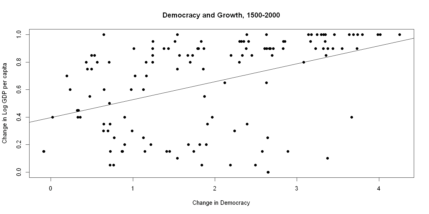
16.3.3. Figure 16.1

plot(growth, democracy, xlab="Change in Democracy", 
    ylab="Change in Log GDP per capita", 
     main="Democracy and Growth, 1500-2000", pch=19)
abline(ols.bivariate)

Multiple regression

ols.multiple = lm(democracy ~ growth+constraint+indcent+catholic+muslim+protestant)
summ(ols.multiple, digits=3, robust = "HC1")

MODEL INFO:
Observations: 131
Dependent Variable: democracy
Type: OLS linear regression 

MODEL FIT:
F(6,124) = 16.858, p = 0.000
R² = 0.449
Adj. R² = 0.423 

Standard errors: Robust, type = HC1
---------------------------------------------------
                      Est.    S.E.   t val.       p
----------------- -------- ------- -------- -------
(Intercept)          3.031   0.975    3.109   0.002
growth               0.047   0.025    1.841   0.068
constraint           0.164   0.072    2.270   0.025
indcent             -0.133   0.050   -2.661   0.009
catholic             0.117   0.089    1.324   0.188
muslim              -0.233   0.101   -2.303   0.023
protestant           0.180   0.104    1.732   0.086
---------------------------------------------------

16.4. 16.8 DIAGNOSTICS

yhat = predict(ols.multiple)
uhat = resid(ols.multiple)

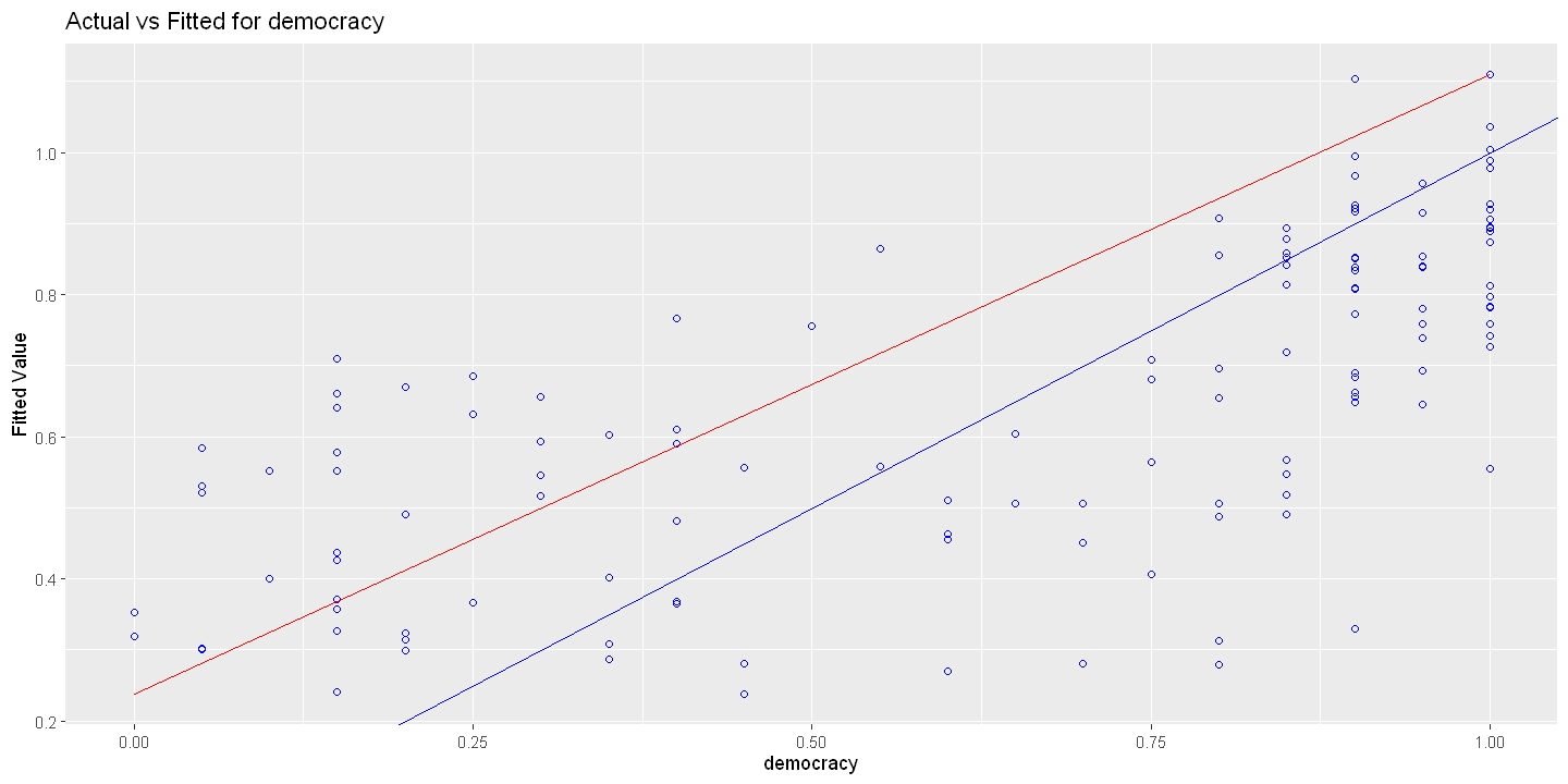
16.4.1. Figure 16.2 using olsrr package

Actual versus fitted

ols_plot_obs_fit(ols.multiple) 

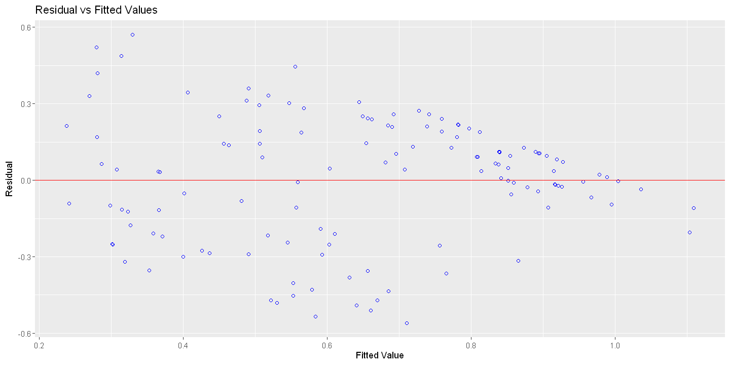
Residual versus fitted

ols_plot_resid_fit(ols.multiple) 

16.4.2. Figure 16.2 - Manually

Panel A Actual vs. Fitted

plot(yhat, democracy, xlab="Predicted value of y", ylab="Actual value of y", 
    main="Actual vs. Fitted", pch=19)
ols.actvsfitted = lm(democracy ~ yhat)
abline(ols.actvsfitted)
lines(lowess(yhat, democracy), lty=3)

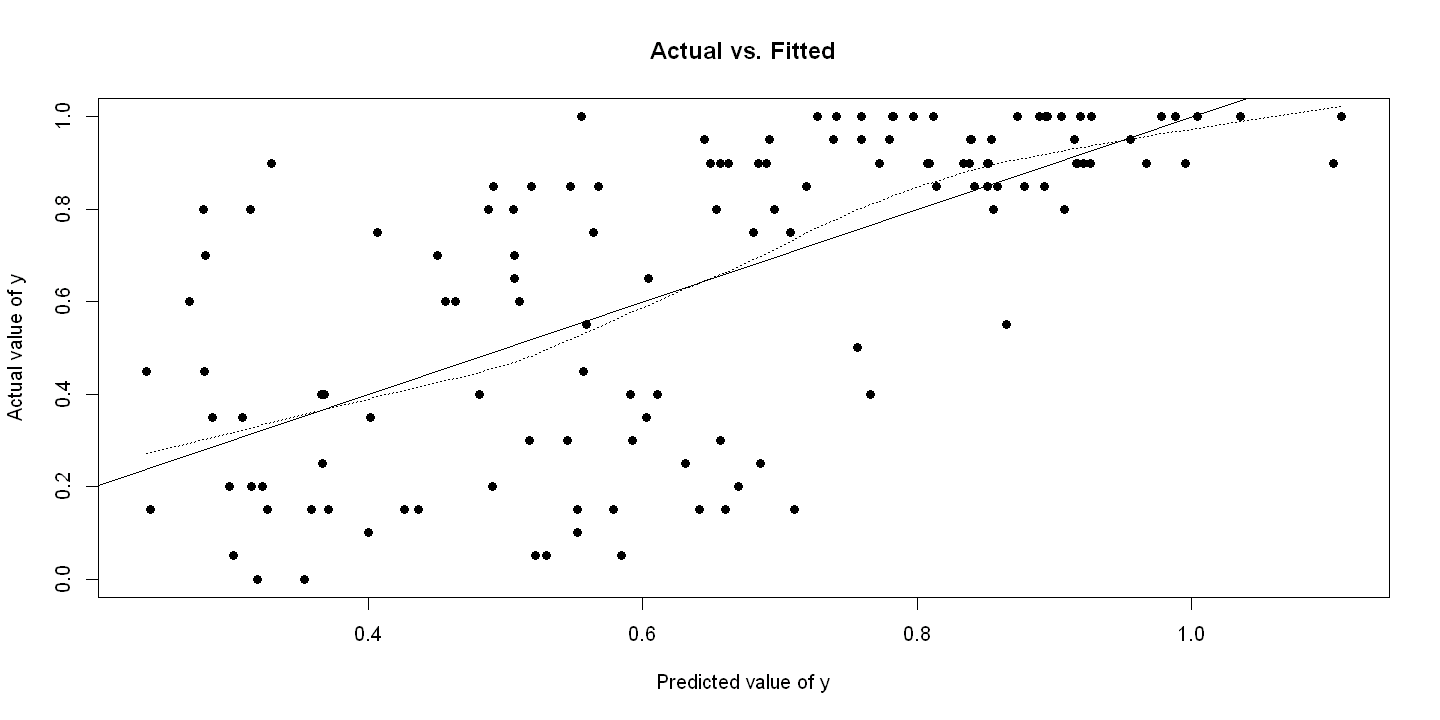
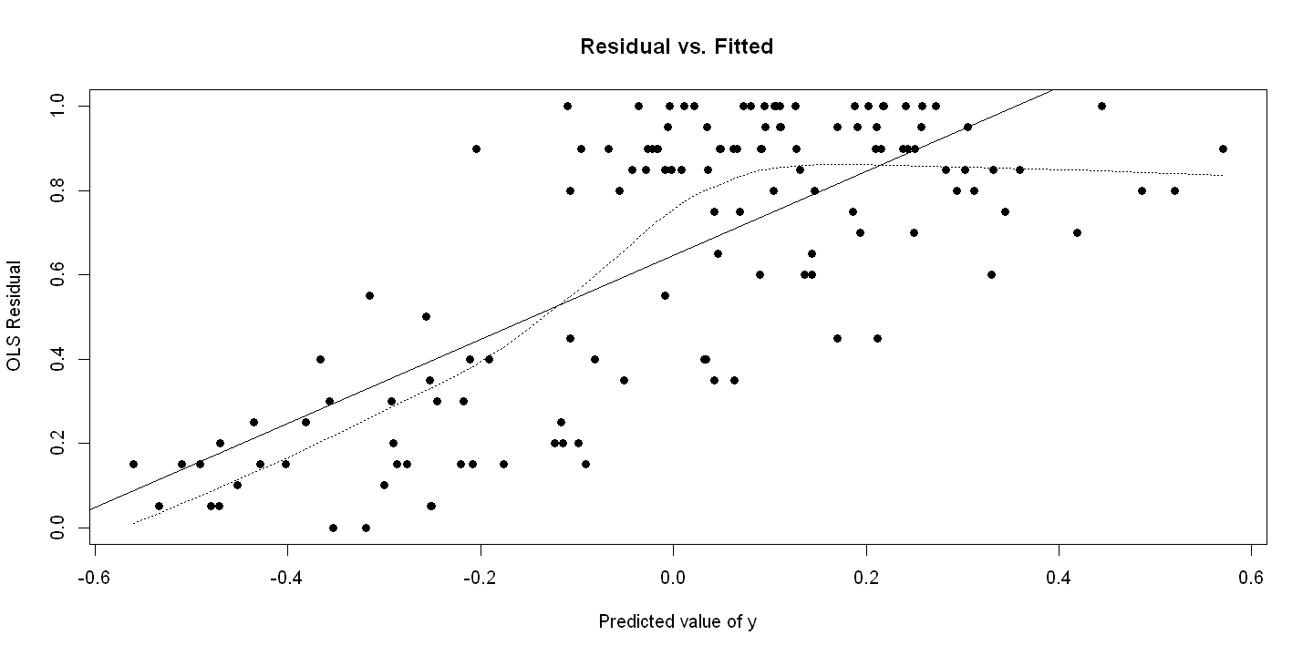
Figure 16.2 - Panel B Residual vs. Fitted

plot(uhat, democracy, xlab="Predicted value of y", ylab="OLS Residual", 
    main="Residual vs. Fitted", pch=19)
ols.residvsfitted = lm(democracy ~ uhat)
abline(ols.residvsfitted)
abline(ols.multiple)
lines(lowess(uhat, democracy), lty=3)

Warning message in abline(ols.multiple):
"only using the first two of 7 regression coefficients"

16.4.3. Figure 16.3

16.4.3.1. Figure 16.3 Using olsrr package for all regressors

Residual versus Regressor - Not available

Figure 16.3 - Panel B Component plus residual plot

ols_plot_comp_plus_resid(ols.multiple)

`geom_smooth()` using formula = 'y ~ x'

`geom_smooth()` using formula = 'y ~ x'

`geom_smooth()` using formula = 'y ~ x'

`geom_smooth()` using formula = 'y ~ x'

`geom_smooth()` using formula = 'y ~ x'

`geom_smooth()` using formula = 'y ~ x'

[[1]]
NULL

[[2]]
NULL

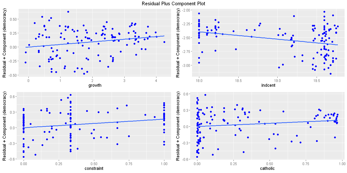
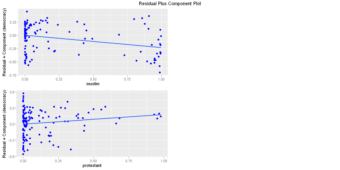
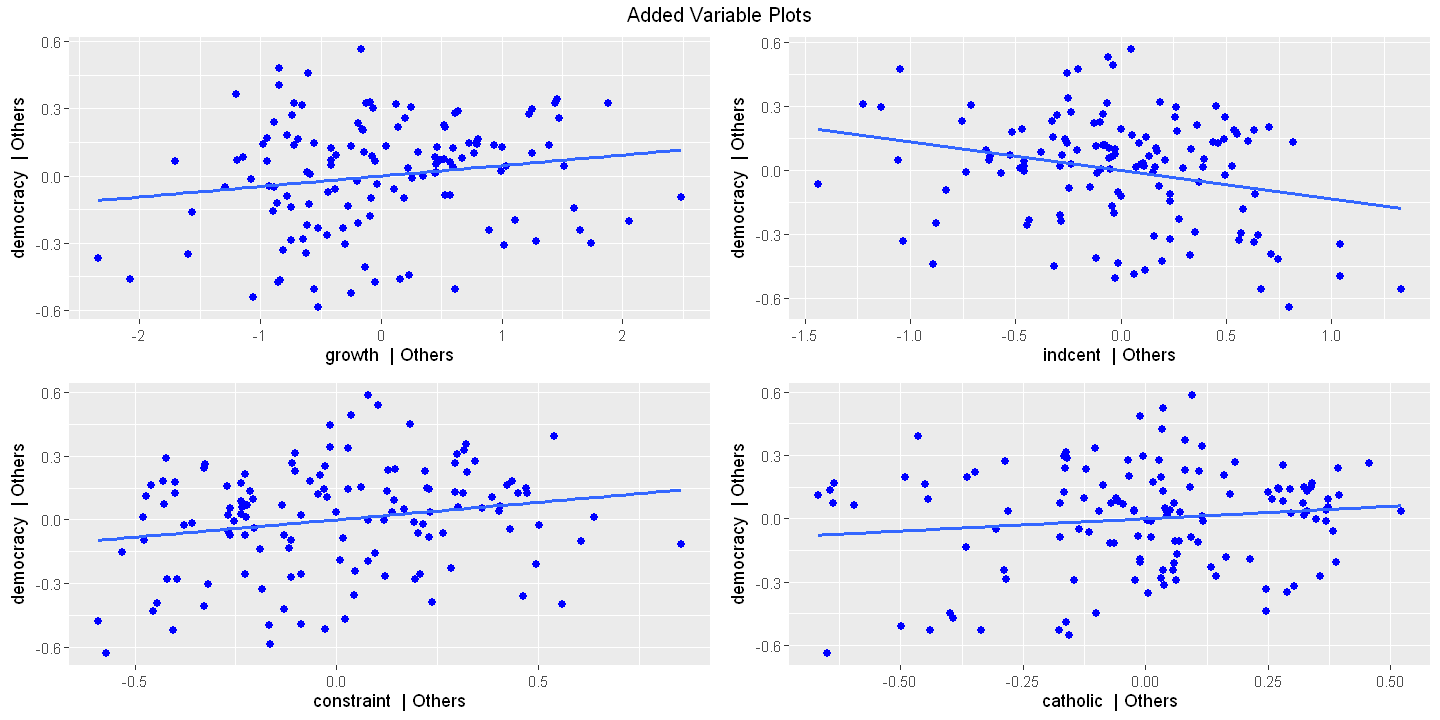
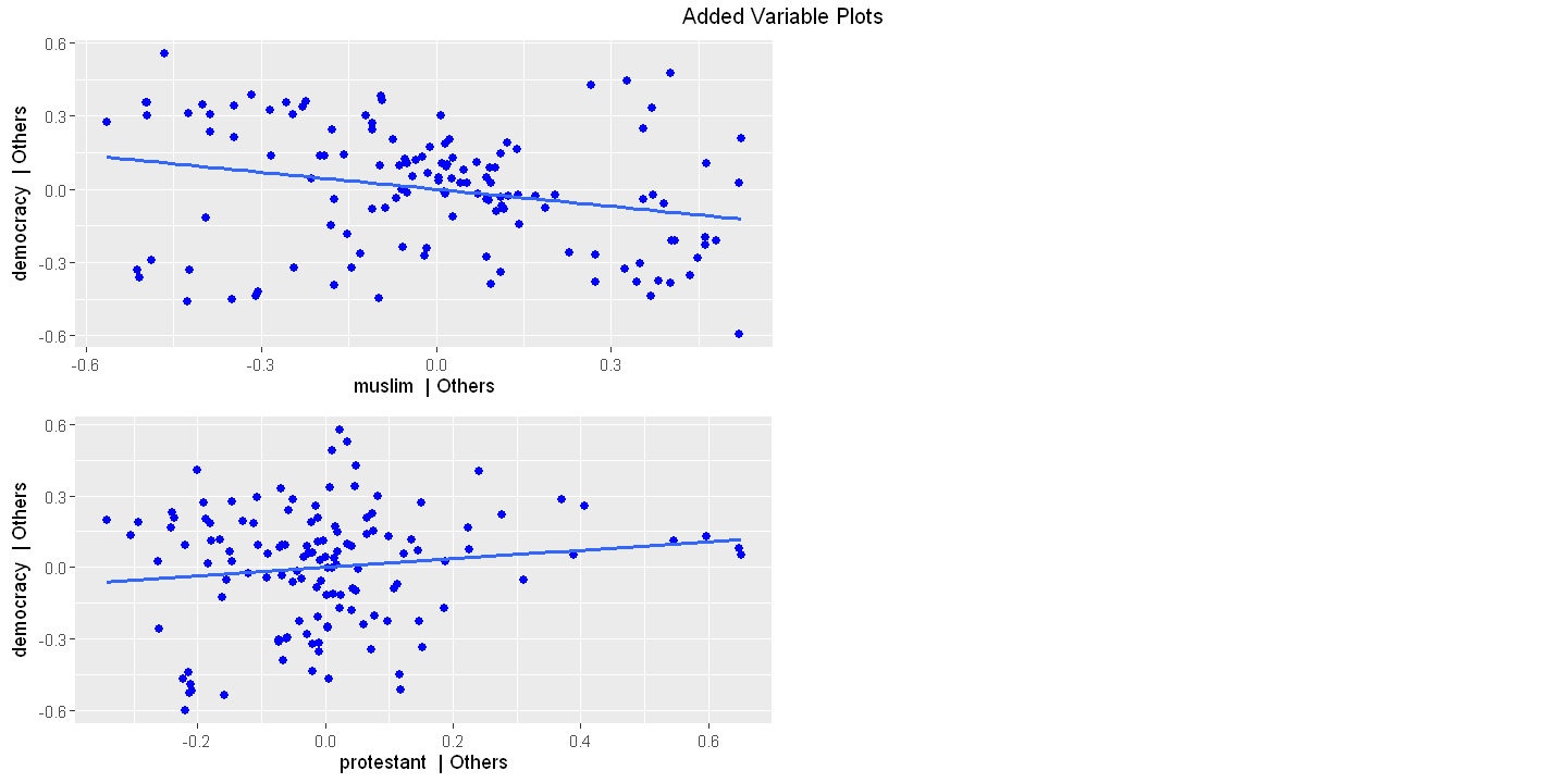
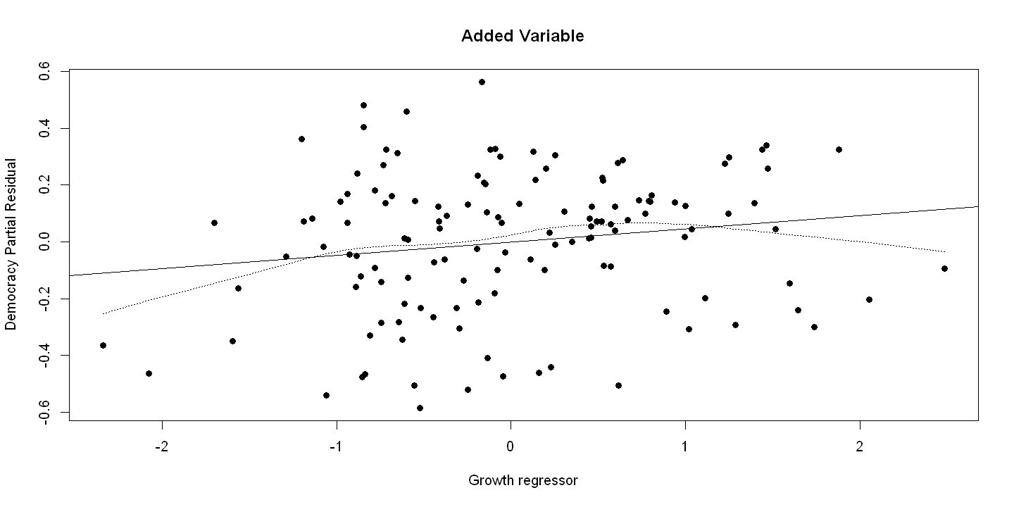
Figure 16.3 - Panel C Added variable plot

ols_plot_added_variable(ols.multiple)

`geom_smooth()` using formula = 'y ~ x'

`geom_smooth()` using formula = 'y ~ x'

`geom_smooth()` using formula = 'y ~ x'

`geom_smooth()` using formula = 'y ~ x'

`geom_smooth()` using formula = 'y ~ x'

`geom_smooth()` using formula = 'y ~ x'

[[1]]
NULL

[[2]]
NULL

16.4.3.2. Figure 16.3 done manually for a single regressor growth

Figure 16.3 - Panel A Residual versus Regressor

plot(growth, uhat, xlab="Growth regressor", ylab="Democracy Residual", 
    main="Residual versus Regressor", pch=19)
abline(h=0)
lines(lowess(growth, uhat), lty=3)

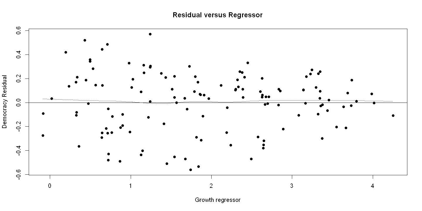
Figure 16.3 - Panel B Component plus residual plot

bgrowth=summary(ols.multiple)$coefficients["growth",1]
prgrowth = bgrowth*growth + uhat
ols.compplusres = lm(prgrowth ~ growth)
plot(growth, prgrowth, xlab="Growth regressor", ylab="Dem Res + .049*Growth", 
    main="Component Plus Residual", pch=19)
abline(ols.compplusres)
lines(lowess(growth, prgrowth), lty=3)

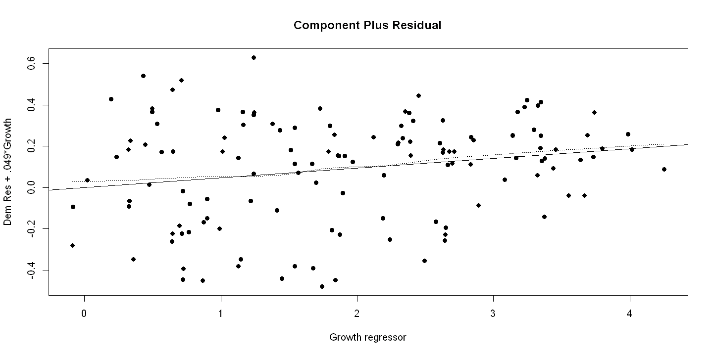
Figure 16.3 - Panel C Added variable plot done manually

Drop growth from regression model

ols.nogrowth = lm(democracy ~ constraint+indcent+catholic+muslim+protestant)
uhat1democ = resid(ols.nogrowth)

Growth is dependent variable

ols.growth = lm(growth ~ constraint+indcent+catholic+muslim+protestant)
uhat1growth = resid(ols.growth)
ols.addedvar = lm(uhat1democ ~ uhat1growth)
plot(uhat1growth, uhat1democ, xlab="Growth regressor", ylab="Democracy Partial Residual", 
    main="Added Variable", pch=19)
abline(ols.addedvar)
lines(lowess(uhat1growth, uhat1democ), lty=3)

Influential Observations using library(olsrr)

ols.multiple = lm(democracy ~ growth+constraint+indcent+catholic+muslim+protestant)

DFITS

Plot

ols_plot_dffits(ols.multiple)

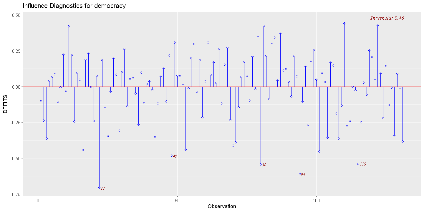
List the threshold and large DFITS

dfits = ols_plot_dffits(ols.multiple, print_plot= FALSE)
print(dfits$threshold)
print(dfits$outliers)
summary(dfits$outliers)

[1] 0.46

    observation     dffits
22           22 -0.7041223
48           48 -0.4812355
80           80 -0.5427028
94           94 -0.6105840
115         115 -0.5377741

  observation        dffits       
 Min.   : 22.0   Min.   :-0.7041  
 1st Qu.: 48.0   1st Qu.:-0.6106  
 Median : 80.0   Median :-0.5427  
 Mean   : 71.8   Mean   :-0.5753  
 3rd Qu.: 94.0   3rd Qu.:-0.5378  
 Max.   :115.0   Max.   :-0.4812  

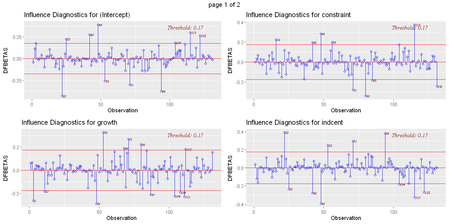
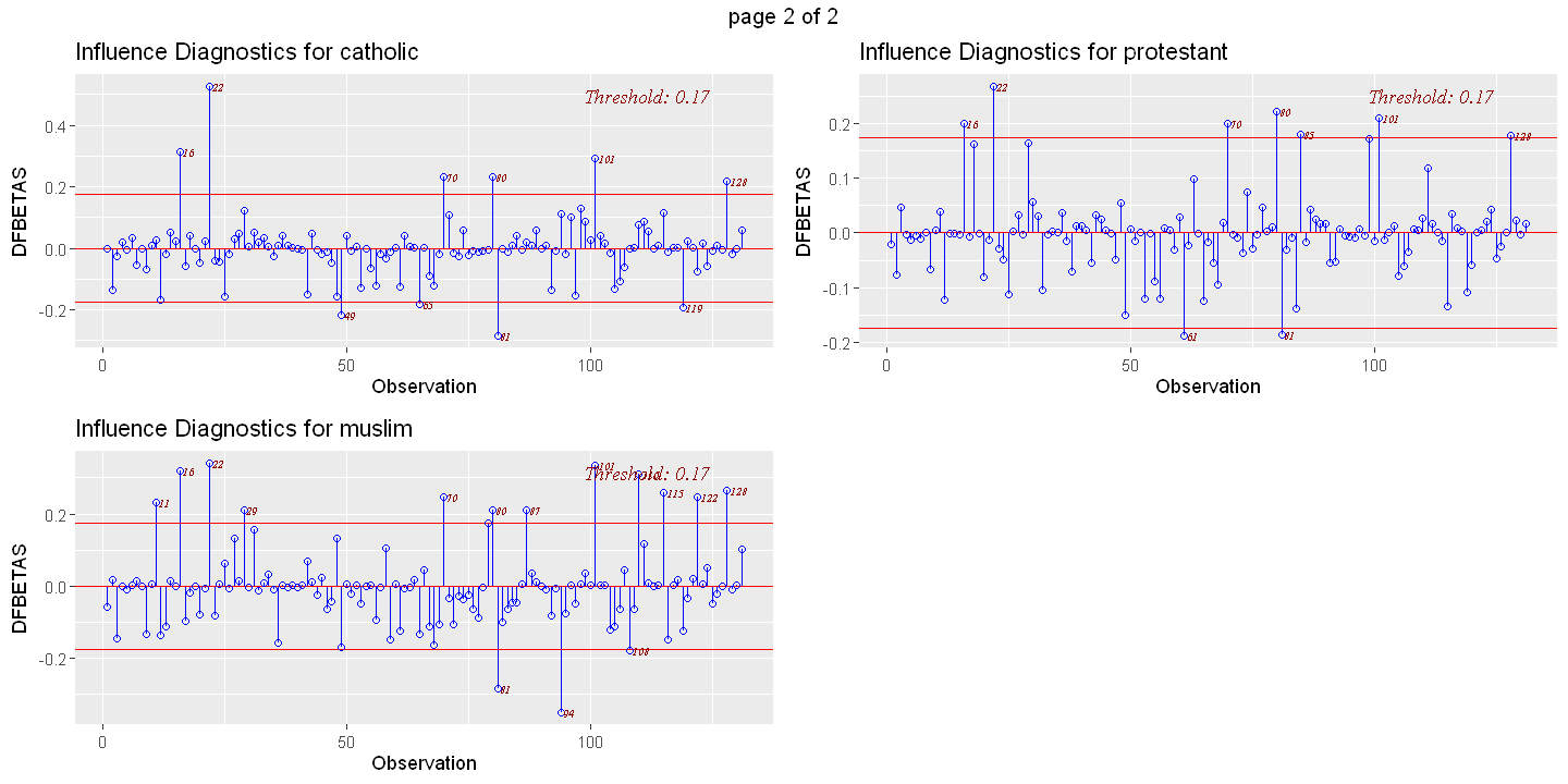
DFBETAS - Separate plots for each regressor

ols_plot_dfbetas(ols.multiple)
dfbetas = ols_plot_dfbetas(ols.multiple, print_plot= FALSE)

[[1]]
NULL

[[2]]
NULL