4. CHAPTER 4. STATISTICAL INFERENCE FOR THE MEAN#
SET UP
library(foreign) # to open stata.dta files
library(psych) # for better sammary of descriptive statistics
library(repr) # to combine graphs with adjustable plot dimensions
options(repr.plot.width = 12, repr.plot.height = 6) # Plot dimensions (in inches)
options(width = 150) # To increase character width of printed output
4.1. 4.1 EXAMPLE: MEAN ANNUAL EARNINGS#
df.earn = read.dta(file = "Dataset/AED_EARNINGS.DTA")
print((describe(df.earn)))
          vars   n     mean       sd median  trimmed      mad  min    max  range  skew kurtosis      se
earnings     1 171 41412.69 25527.05  36000 38052.70 17049.90 1050 172000 170950  1.70     4.23 1952.10
education    2 171    14.43     2.74     14    14.45     2.97    3     20     17 -0.45     1.16    0.21
age          3 171    30.00     0.00     30    30.00     0.00   30     30      0   NaN      NaN    0.00
gender       4 171     0.00     0.00      0     0.00     0.00    0      0      0   NaN      NaN    0.00
# Summary statisitcs
attach(df.earn)
summary(earnings)
sd(earnings)
   Min. 1st Qu.  Median    Mean 3rd Qu.    Max.
   1050   25000   36000   41413   49000  172000
25527.0533958379
# 95% Confidence interval
t.test(earnings)$"conf.int"
- 37559.20698453
- 45266.1731324291
# Hypothesis test
t.test(earnings, mu=40000)
	One Sample t-test

data:  earnings
t = 0.72368, df = 170, p-value = 0.4703
alternative hypothesis: true mean is not equal to 40000
95 percent confidence interval:
 37559.21 45266.17
sample estimates:
mean of x
 41412.69
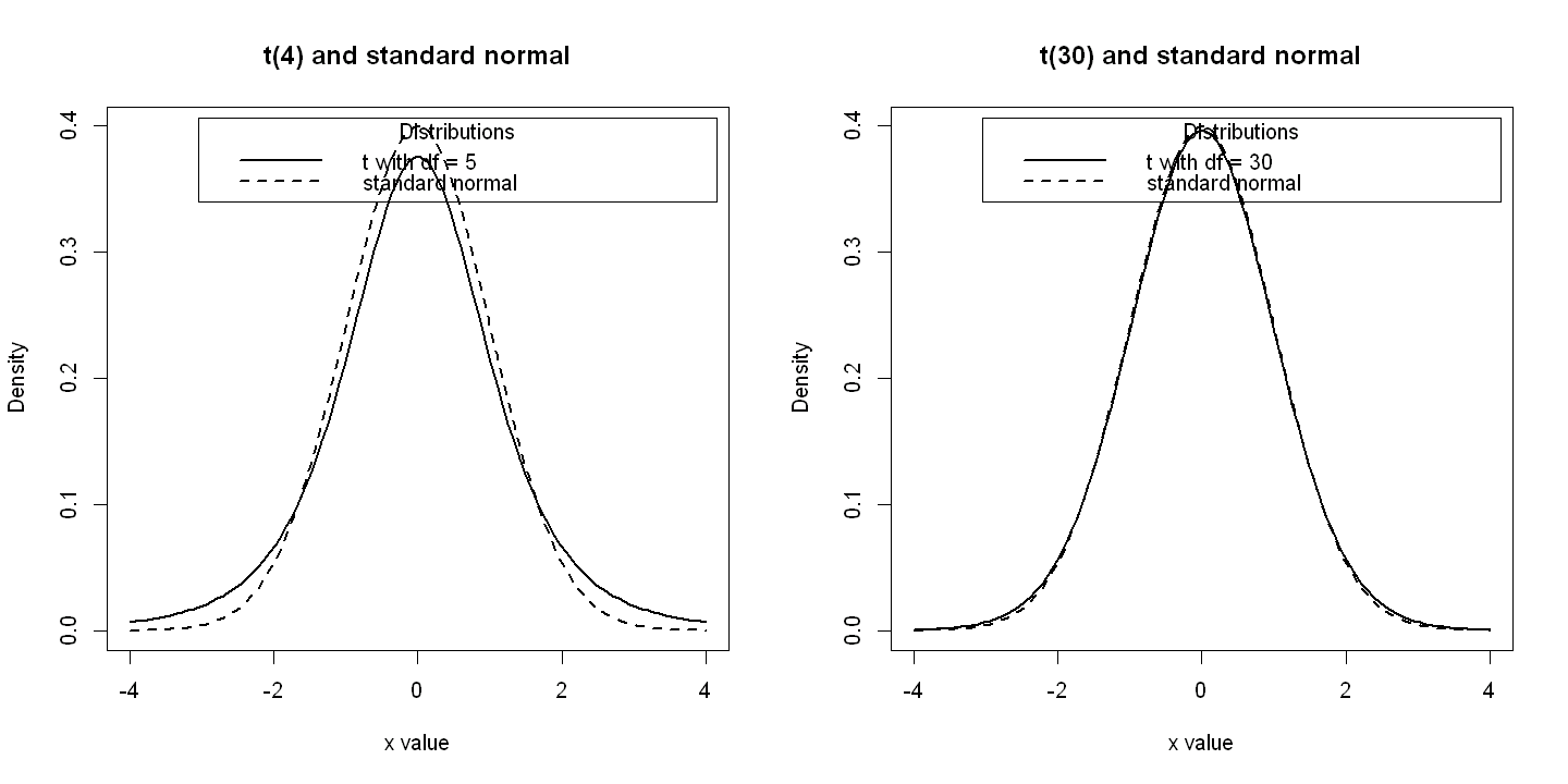
4.2. 4.2 t Statistic and t DISTRIBUTION#
# Plot standard normal and t densities with 4 and 30 degrees of freedom

par(mfrow=c(1,2)) # Combine both panels in one row, two column

# Panel A  t(4) and standard normal
x <- seq(-4, 4, length=100)
hx <- dnorm(x)
labels <- c("t with df = 5", "standard normal")
plot(x, hx, type="l", lty=2, lwd=2, xlab="x value",
     ylab="Density", main="t(4) and standard normal")
lines(x, dt(x,4), lty=1, lwd=2)
legend("topright", inset=.02, title="Distributions",
       labels, lwd=2, lty=c(1, 2))

# Panel B  t(30) and standard normal
labels <- c("t with df = 30", "standard normal")
plot(x, hx, type="l", lty=2, lwd=2, xlab="x value",
     ylab="Density", main="t(30) and standard normal")
lines(x, dt(x,30), lty=1, lwd=2)
legend("topright", inset=.02, title="Distributions",
       labels, lwd=2, lty=c(1, 2))
4.3. 4.3 CONFIDENCE INTERVALS#
summary(earnings)

# 95% Confidence interval
t.test(earnings)$"conf.int"
   Min. 1st Qu.  Median    Mean 3rd Qu.    Max.
   1050   25000   36000   41413   49000  172000
- 37559.20698453
- 45266.1731324291
# 90% and 99% confidence intervals
t.test(earnings, conf.level=0.90)$"conf.int"
t.test(earnings, conf.level=0.99)$"conf.int"
- 38184.1733816741
- 44641.206735285
- 36327.3489591822
- 46498.0311577768
# Confidence interval manually
mean = mean(earnings)
sd = sd(earnings)
N = length(earnings)
sterror = sd/sqrt(N)
tcrit = qt(.975,N-1)
intwidth = tcrit*sterror
print("95% confidence interval = ")
cbind(mean - intwidth, mean + intwidth)
[1] "95% confidence interval = "
| 37559.21 | 45266.17 |
4.4. 4.4 TWO-SIDED HYPOTHESIS TEST#
# Test H0: mu = 40000 against HA: mu not = 40000
t.test(earnings, mu = 40000)
	One Sample t-test

data:  earnings
t = 0.72368, df = 170, p-value = 0.4703
alternative hypothesis: true mean is not equal to 40000
95 percent confidence interval:
 37559.21 45266.17
sample estimates:
mean of x
 41412.69
# Same two-sided test done manually
mu0 = 40000
mean = mean(earnings)
sd = sd(earnings)
N = length(earnings)
sterror = sd/sqrt(N)
t = (mean-mu0)/sterror
p = 2*(1-pt(abs(t),N-1))
# Equivalent is 2*pt(t,N-1,lower.tail=FALSE)
tcrit = qt(.975,N-1)
print("t statistic, p-value, critical value")
cbind(t, p, tcrit)
[1] "t statistic, p-value, critical value"
| t | p | tcrit |
|---|---|---|
| 0.7236761 | 0.4702592 | 1.974017 |
4.5. 4.5 TWO-SIDED HYPOTHESIS TEST EXAMPLES#
# Gasoline price September 2 2013 from sactogasprices.com part of GasBuddy.com
rm(list=ls())
library(foreign)
df = read.dta(file = "Dataset/AED_GASPRICE.DTA")
attach(df)
print((describe(df)))
summary(price)
      vars  n mean   sd median trimmed  mad  min  max range skew kurtosis   se
city*    1 32 1.91 0.73   2.00    1.88 1.48 1.00 3.00   2.0 0.14    -1.20 0.13
price    2 32 3.67 0.15   3.65    3.65 0.18 3.49 4.09   0.6 0.71     0.14 0.03
   Min. 1st Qu.  Median    Mean 3rd Qu.    Max.
   3.49    3.55    3.65    3.67    3.79    4.09
# Test H0: mu = 3.81 against HA: mu not = 50000
t.test(price, mu = 3.81)
t = (3.6697-3.81)/(0.1510/sqrt(32))
p = 2*(1-pt(abs(t),31))
tcrit = qt(.975,31)
cbind(t, p, tcrit)
	One Sample t-test

data:  price
t = -5.2577, df = 31, p-value = 1.026e-05
alternative hypothesis: true mean is not equal to 3.81
95 percent confidence interval:
 3.615259 3.724116
sample estimates:
mean of x
 3.669687
| t | p | tcrit |
|---|---|---|
| -5.256004 | 1.03076e-05 | 2.039513 |
# Male Earnings 2010 30 year old full time workers
df = read.dta(file = "Dataset/AED_EARNINGSMALE.DTA")
attach(df)
print((describe(df)))
summary(earnings)
The following objects are masked from df.earn:

    age, earnings, education, gender
          vars   n     mean       sd median  trimmed      mad min    max  range  skew kurtosis      se
earnings     1 191 52353.93 65034.74  38000 41328.76 20756.40   1 498000 497999  5.31    32.38 4705.75
education    2 191    13.43     3.01     13    13.55     1.48   0     20     20 -1.12     3.95    0.22
age          3 191    30.00     0.00     30    30.00     0.00  30     30      0   NaN      NaN    0.00
gender       4 191     1.00     0.00      1     1.00     0.00   1      1      0   NaN      NaN    0.00
   Min. 1st Qu.  Median    Mean 3rd Qu.    Max.
      1   25500   38000   52354   58850  498000
# Test H0: mu = 50000 against HA: mu not = 50000
t.test(earnings, mu=50000)
t = (52353.93-50000)/(65034.74/sqrt(191))
p = 2*(1-pt(abs(t),190))
tcrit= qt(.975,190)
cbind(t, p, tcrit)
	One Sample t-test

data:  earnings
t = 0.50022, df = 190, p-value = 0.6175
alternative hypothesis: true mean is not equal to 50000
95 percent confidence interval:
 43071.71 61636.15
sample estimates:
mean of x
 52353.93
| t | p | tcrit |
|---|---|---|
| 0.5002243 | 0.617496 | 1.972528 |
# Growth in real GDP per capita
# Read in the Stata data set - requires package foreign
df = read.dta(file = "Dataset/AED_REALGDPPC.DTA")
attach(df)
print((describe(df)))
summary(growth)
Warning message in FUN(newX[, i], ...):
"no non-missing arguments to min; returning Inf"
Warning message in FUN(newX[, i], ...):
"no non-missing arguments to max; returning -Inf"
          vars   n      mean       sd    median   trimmed      mad       min       max     range  skew kurtosis      se
gdpc1        1 245   9925.24  4814.02   9238.92   9716.91  6140.55   3121.94  19221.97  16100.03  0.32    -1.25  307.56
gdp          2 245   7401.46  6331.00   5695.36   6755.00  6885.44    510.33  21729.12  21218.79  0.65    -0.88  404.47
gdpdef       3 245     59.72    31.20     61.65     59.06    44.57     16.35    113.50     97.16  0.03    -1.36    1.99
date*        4 245    123.00    70.87    123.00    123.00    90.44      1.00    245.00    244.00  0.00    -1.21    4.53
daten        5 245       NaN       NA        NA       NaN       NA       Inf      -Inf      -Inf    NA       NA      NA
quarter      6 245    118.00    70.87    118.00    118.00    90.44     -4.00    240.00    244.00  0.00    -1.21    4.53
popthm       7 245 253116.88 45611.79 247695.00 252742.75 58854.77 176044.00 329527.00 153483.00  0.10    -1.28 2914.03
year         8 245   1989.13    17.72   1989.00   1989.13    22.24   1959.00   2020.00     61.00  0.00    -1.21    1.13
realgdp      9 245   9925.24  4814.03   9238.97   9716.90  6140.78   3121.86  19222.00  16100.14  0.32    -1.25  307.56
gdppc       10 245  25841.47 19184.69  22993.15  24423.21 24740.38   2898.86  66008.59  63109.73  0.44    -1.13 1225.66
realgdppc   11 245  37050.50 12089.68  36929.01  36996.63 16507.15  17733.26  58392.45  40659.20  0.08    -1.33  772.38
growth      12 241      1.99     2.18      2.09      2.08     1.80     -4.77      7.63     12.40 -0.38     0.64    0.14
   Min. 1st Qu.  Median    Mean 3rd Qu.    Max.    NA's
-4.7722  0.8924  2.0896  1.9905  3.3142  7.6305       4
# Test H0: mu = 2.0 against HA: mu not = 2.0
t.test(growth, mu=2.0)
t = (1.9904-2.0)/(2.1781/sqrt(241))
p = 2*(1-pt(abs(t),241))
tcrit= qt(.975,241)
cbind(t, p, tcrit)
	One Sample t-test

data:  growth
t = -0.068021, df = 240, p-value = 0.9458
alternative hypothesis: true mean is not equal to 2
95 percent confidence interval:
 1.714073 2.266840
sample estimates:
mean of x
 1.990456
| t | p | tcrit |
|---|---|---|
| -0.06842297 | 0.9455057 | 1.969856 |
4.6. 4.6 ONE-SIDED DIRECTIONAL HYPOTHESIS TESTS#
t.test(earnings, mu=50000, alternative = "less")
	One Sample t-test

data:  earnings
t = 0.50022, df = 190, p-value = 0.6913
alternative hypothesis: true mean is less than 50000
95 percent confidence interval:
     -Inf 60132.12
sample estimates:
mean of x
 52353.93
df.earn = read.dta(file = "Dataset/AED_EARNINGS.DTA")
attach(df.earn)
print((describe(df.earn)))
summary(earnings)
The following objects are masked from df (pos = 4):

    age, earnings, education, gender
The following objects are masked from df.earn (pos = 6):

    age, earnings, education, gender
          vars   n     mean       sd median  trimmed      mad  min    max  range  skew kurtosis      se
earnings     1 171 41412.69 25527.05  36000 38052.70 17049.90 1050 172000 170950  1.70     4.23 1952.10
education    2 171    14.43     2.74     14    14.45     2.97    3     20     17 -0.45     1.16    0.21
age          3 171    30.00     0.00     30    30.00     0.00   30     30      0   NaN      NaN    0.00
gender       4 171     0.00     0.00      0     0.00     0.00    0      0      0   NaN      NaN    0.00
   Min. 1st Qu.  Median    Mean 3rd Qu.    Max.
   1050   25000   36000   41413   49000  172000
# Test H0: mu < 40000 against HA: mu >= 40000 using Stata command ttest
t.test(earnings, mu=40000, alternative = "greater")
	One Sample t-test

data:  earnings
t = 0.72368, df = 170, p-value = 0.2351
alternative hypothesis: true mean is greater than 40000
95 percent confidence interval:
 38184.17      Inf
sample estimates:
mean of x
 41412.69
# Same two-sided test done manually
mu0 = 40000
mean = mean(earnings)
sd = sd(earnings)
N = length(earnings)
sterror = sd/sqrt(N)
t = (mean-mu0)/sterror
p = 1-pt(abs(t),N-1)
# Equivalent is pt(t,N-1,lower.tail=FALSE)
tcrit = qt(.95,N-1)
print("t statistic, p-value, critical value")
cbind(t, p, tcrit)
[1] "t statistic, p-value, critical value"
| t | p | tcrit |
|---|---|---|
| 0.7236761 | 0.2351296 | 1.653866 |
4.7. 4.8 PROPORTIONS DATA#
# Confidence interval
mean = (480*1+441*0)/921
sterror = sqrt( (mean*(1-mean)) / 921)
print("mean and standard error")
cbind(mean, sterror)
print("95% CI")
cbind(mean-1.964*sterror, mean+1.964*sterror)
[1] "mean and standard error"
| mean | sterror |
|---|---|
| 0.5211726 | 0.01646078 |
[1] "95% CI"
| 0.4888437 | 0.5535016 |
# Test mu = 0.50
sterrorH0 = sqrt( (0.5*(1-0.5)) / 921)
t = (mean - 0.5) / sterrorH0
p = 2*(1-pnorm(abs(t)))
print("t statistic, p-value, critical value")
cbind(t, p, tcrit)
[1] "t statistic, p-value, critical value"
| t | p | tcrit |
|---|---|---|
| 1.285094 | 0.1987595 | 1.653866 |