9. CHAPTER 09. MODELS WITH NATURAL LOGARITHMS#
SET UP
library(foreign) # to open stata.dta files
library(psych) # for better sammary of descriptive statistics
library(repr) # to combine graphs with adjustable plot dimensions
options(repr.plot.width = 12, repr.plot.height = 6) # Plot dimensions (in inches)
options(width = 150) # To increase character width of printed output
9.1. 9.4 EXAMPLE: EARNINGS AND EDUCATION#
df = read.dta(file = "Dataset/AED_EARNINGS.DTA")
attach(df)
print(describe(df))
print(head(df))
          vars   n     mean       sd median  trimmed      mad  min    max  range  skew kurtosis      se
earnings     1 171 41412.69 25527.05  36000 38052.70 17049.90 1050 172000 170950  1.70     4.23 1952.10
education    2 171    14.43     2.74     14    14.45     2.97    3     20     17 -0.45     1.16    0.21
age          3 171    30.00     0.00     30    30.00     0.00   30     30      0   NaN      NaN    0.00
gender       4 171     0.00     0.00      0     0.00     0.00    0      0      0   NaN      NaN    0.00
  earnings education age gender
1    25000        14  30      0
2    40000        12  30      0
3    25000        13  30      0
4    38000        13  30      0
5    28800        12  30      0
6    31000        16  30      0
Create variables and add to data frame
lnearn = log(earnings)
df$lnearn = lnearn
lneduc = log(education)
df$lneduc = lneduc
9.1.1. Table 9.2#
table92vars = c("earnings", "lnearn", "education", "lneduc")
print(describe(df[table92vars]))
          vars   n     mean       sd   median  trimmed      mad     min       max    range  skew kurtosis      se
earnings     1 171 41412.69 25527.05 36000.00 38052.70 17049.90 1050.00 172000.00 170950.0  1.70     4.23 1952.10
lnearn       2 171    10.46     0.62    10.49    10.47     0.54    6.96     12.06      5.1 -0.90     4.74    0.05
education    3 171    14.43     2.74    14.00    14.45     2.97    3.00     20.00     17.0 -0.45     1.16    0.21
lneduc       4 171     2.65     0.22     2.64     2.66     0.20    1.10      3.00      1.9 -2.42    13.27    0.02
9.1.2. Table 9.3#
Linear model
ols.linear <- lm(earnings ~ education)
library(jtools)
summ(ols.linear, digits=3)
MODEL INFO:
Observations: 171
Dependent Variable: earnings
Type: OLS linear regression

MODEL FIT:
F(1,169) = 68.857, p = 0.000
R² = 0.289
Adj. R² = 0.285

Standard errors:OLS
----------------------------------------------------------
                          Est.       S.E.   t val.       p
----------------- ------------ ---------- -------- -------
(Intercept)         -31055.915   8887.835   -3.494   0.001
education             5021.123    605.101    8.298   0.000
----------------------------------------------------------
Log-linear Model
summ(ols.loglin <- lm(lnearn ~ education), digits=3)
MODEL INFO:
Observations: 171
Dependent Variable: lnearn
Type: OLS linear regression

MODEL FIT:
F(1,169) = 84.743, p = 0.000
R² = 0.334
Adj. R² = 0.330

Standard errors:OLS
--------------------------------------------------
                     Est.    S.E.   t val.       p
----------------- ------- ------- -------- -------
(Intercept)         8.561   0.210   40.825   0.000
education           0.131   0.014    9.206   0.000
--------------------------------------------------
Log-log Model
summ(ols.loglog <- lm(lnearn ~ lneduc), digits=3)
MODEL INFO:
Observations: 171
Dependent Variable: lnearn
Type: OLS linear regression

MODEL FIT:
F(1,169) = 67.668, p = 0.000
R² = 0.286
Adj. R² = 0.282

Standard errors:OLS
--------------------------------------------------
                     Est.    S.E.   t val.       p
----------------- ------- ------- -------- -------
(Intercept)         6.543   0.478   13.700   0.000
lneduc              1.478   0.180    8.226   0.000
--------------------------------------------------
Linear-log Model
summ(ols.linlog <- lm(earnings ~ lneduc), digits=3)
MODEL INFO:
Observations: 171
Dependent Variable: earnings
Type: OLS linear regression

MODEL FIT:
F(1,169) = 50.570, p = 0.000
R² = 0.230
Adj. R² = 0.226

Standard errors:OLS
------------------------------------------------------------
                           Est.        S.E.   t val.       p
----------------- ------------- ----------- -------- -------
(Intercept)         -102767.278   20347.617   -5.051   0.000
lneduc                54452.483    7657.259    7.111   0.000
------------------------------------------------------------
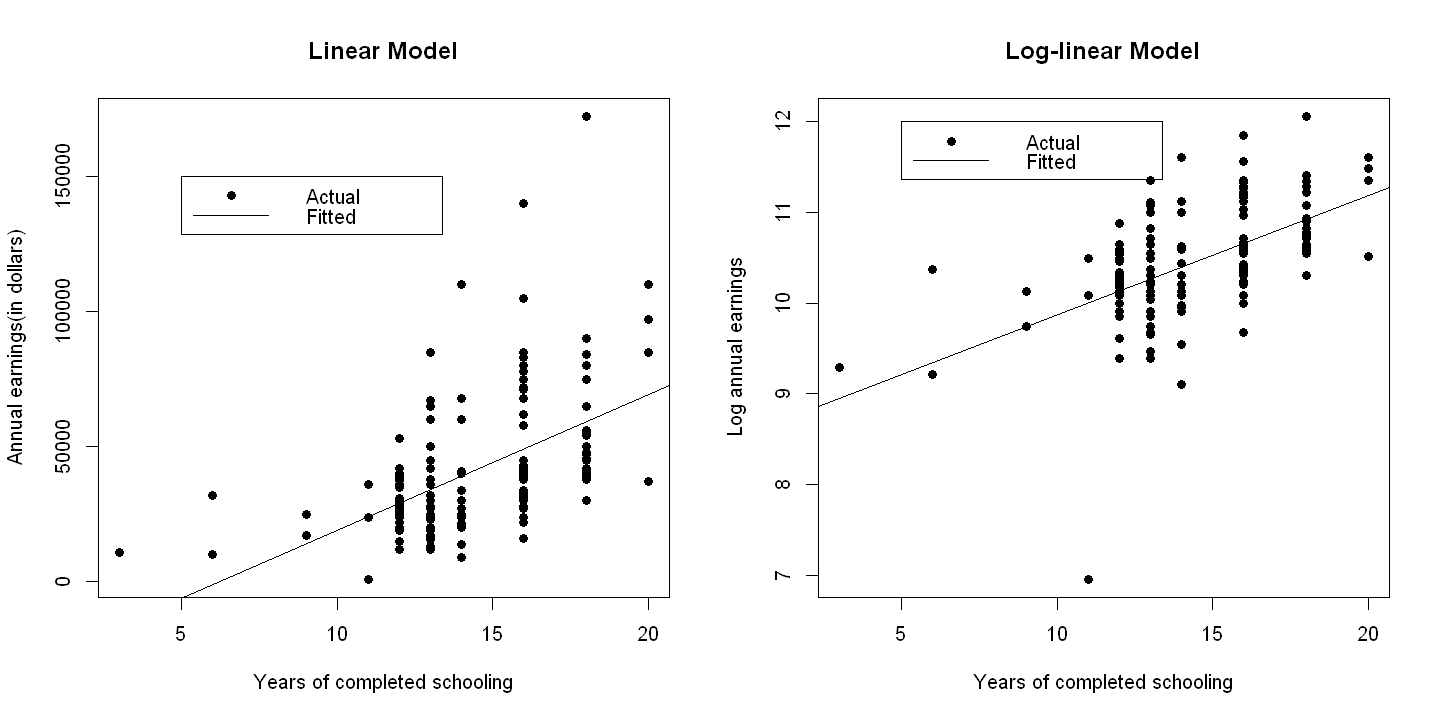
9.1.3. Figure 9.1#
par(mfrow = c(1,2))
# first panel
plot(education,earnings, xlab="Years of completed schooling",
    ylab="Annual earnings(in dollars)",pch=19,main="Linear Model")
abline(ols.linear)
legend(5, 150000, c("Actual",  "Fitted"), lty=c(-1,1), pch=c(19,-1), bty="o")

# second panel
plot(education,lnearn, xlab="Years of completed schooling",
    ylab="Log annual earnings",pch=19,main="Log-linear Model")
abline(ols.loglin)
legend(5, 12, c("Actual",  "Fitted"), lty=c(-1,1), pch=c(19,-1), bty="o")
9.2. 9.5 FURTHER USES OF THE NATURAL LOGARITHM#
9.2.1. Table 9.5#
rm(list=ls())
df = read.dta(file = "Dataset/AED_SP500INDEX.DTA")
attach(df)
print(describe(df))
print(head(df))
        vars  n    mean     sd  median trimmed    mad     min     max   range skew kurtosis    se
year       1 93 1973.00  26.99 1973.00 1973.00  34.10 1927.00 2019.00   92.00 0.00    -1.24  2.80
sp500      2 93  473.66 710.75   96.47  325.68 123.34    6.92 3230.78 3223.86 1.77     2.58 73.70
lnsp500    3 93    4.82   1.80    4.57    4.79   2.34    1.93    8.08    6.15 0.16    -1.27  0.19
  year sp500  lnsp500
1 1927 17.66 2.871302
2 1928 24.35 3.192532
3 1929 21.45 3.065725
4 1930 15.34 2.730464
5 1931  8.12 2.094330
6 1932  6.92 1.934416
To predict exponential growth in the graph in levels
summ(ols.logs <- lm(lnsp500 ~ year))
plnsp500 = predict(ols.logs)
MODEL INFO:
Observations: 93
Dependent Variable: lnsp500
Type: OLS linear regression

MODEL FIT:
F(1,91) = 2070.52, p = 0.00
R² = 0.96
Adj. R² = 0.96

Standard errors:OLS
--------------------------------------------------
                       Est.   S.E.   t val.      p
----------------- --------- ------ -------- ------
(Intercept)         -124.09   2.83   -43.80   0.00
year                   0.07   0.00    45.50   0.00
--------------------------------------------------
Correct for retransformation bias - see chapter 15.6. First need \(rmse^2\) the square of the root mean squared error. Code here uses knowledge that \(k = 2\)
ResSS = c(crossprod(ols.logs$residuals))
MSE = ResSS / (length(ols.logs$residuals) - 2)
sqrt(MSE)
psp500 = exp(plnsp500)*exp(MSE/2)
MSE
0.371732757916085
0.138185243307899
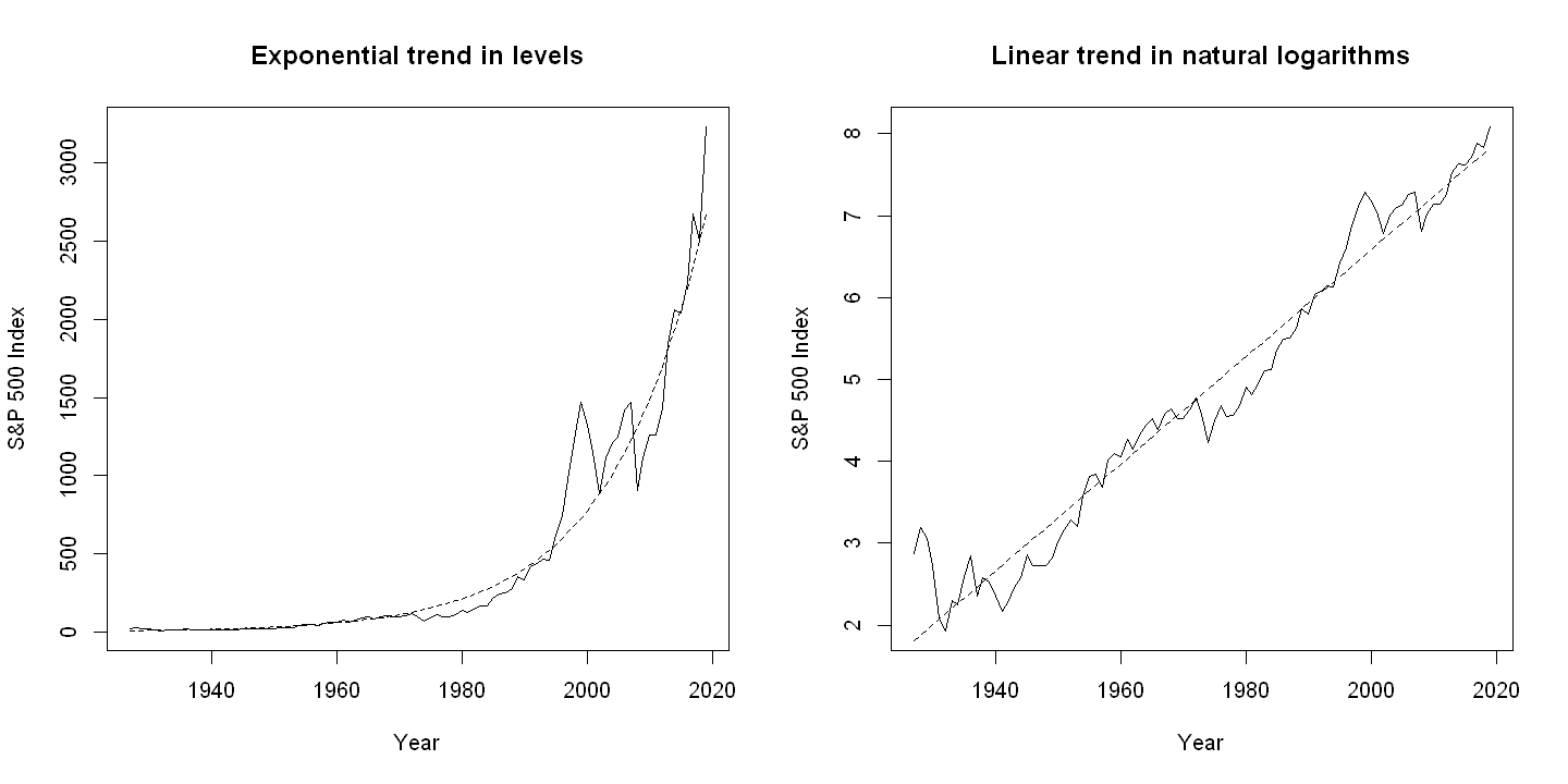
9.2.2. Figure 9.2#
par(mfrow = c(1,2))
# first panel
plot(year, sp500, xlab="Year", ylab="S&P 500 Index", type="l",lty=1,
     main="Exponential trend in levels")
points(year, psp500, type="l",lty=2)
# second panel
plot(year, lnsp500, xlab="Year", ylab="S&P 500 Index", type="l",lty=1,
     main="Linear trend in natural logarithms")
points(year, plnsp500, type="l",lty=2)