12. CHAPTER 12. FURTHER TOPICS IN MULTIPLE REGRESSION#
SET UP
library(foreign) # to open stata.dta files
library(psych) # for better sammary of descriptive statistics
library(repr) # to combine graphs with adjustable plot dimensions
options(repr.plot.width = 12, repr.plot.height = 6) # Plot dimensions (in inches)
options(width = 150) # To increase character width of printed output
12.1. Load Libraries (Packages)#
Show code cell source
pkgs <- c("car", "lmtest", "sandwich","tseries","forecast","bayesreg","psych")
invisible(lapply(pkgs, function(pkg) suppressPackageStartupMessages(library(pkg, character.only = TRUE))))
12.2. 12.1 Inference with Robust Standard Errors#
12.2.1. Load and summarize data#
df <- read.dta("Dataset/AED_HOUSE.DTA")
df_desc<-describe(df)
print(df_desc)
          vars  n      mean       sd median   trimmed      mad    min    max  range  skew kurtosis      se
price        1 29 253910.34 37390.71 244000 249296.00 22239.00 204000 375000 171000  1.48     2.23 6943.28
size         2 29   1882.76   398.27   1800   1836.00   296.52   1400   3300   1900  1.64     3.29   73.96
bedrooms     3 29      3.79     0.68      4      3.72     0.00      3      6      3  0.92     1.89    0.13
bathrooms    4 29      2.21     0.34      2      2.16     0.00      2      3      1  1.28     0.23    0.06
lotsize      5 29      2.14     0.69      2      2.16     0.00      1      3      2 -0.17    -1.00    0.13
age          6 29     36.41     7.12     35     36.20     5.93     23     51     28  0.44    -0.75    1.32
monthsold    7 29      5.97     1.68      6      6.04     1.48      3      8      5 -0.47    -1.03    0.31
list         8 29 257824.14 40860.26 245000 252364.00 23721.60 199900 386000 186100  1.65     2.70 7587.56
12.2.2. Robust SE regression (Table 12.2)#
model <- lm(price ~ size + bedrooms + bathrooms + lotsize + age + monthsold, data = df)
coeftest(model, vcov = vcovHC(model, type = "HC1"))
t test of coefficients:

              Estimate Std. Error t value  Pr(>|t|)
(Intercept) 137791.066  65545.225  2.1022 0.0472030 *
size            68.369     15.359  4.4514 0.0002003 ***
bedrooms      2685.315   8285.528  0.3241 0.7489257
bathrooms     6832.880  19283.791  0.3543 0.7264632
lotsize       2303.221   5328.860  0.4322 0.6697909
age           -833.039    762.930 -1.0919 0.2866932
monthsold    -2088.504   3738.270 -0.5587 0.5820214
---
Signif. codes:  0 '***' 0.001 '**' 0.01 '*' 0.05 '.' 0.1 ' ' 1
12.2.3. HAC SE for mean#
df2 <- read.dta("Dataset/AED_REALGDPPC.dta")
print(describe(df2$growth))

model2 <- lm(growth ~ 1, data = df2)  # mean regression
coeftest(model2, vcov = NeweyWest(model2, lag = 0))  # HAC with lag 0
coeftest(model2, vcov = NeweyWest(model2, lag = 5))  # HAC with lag 5
   vars   n mean   sd median trimmed mad   min  max range  skew kurtosis   se
X1    1 241 1.99 2.18   2.09    2.08 1.8 -4.77 7.63  12.4 -0.38     0.64 0.14
t test of coefficients:

            Estimate Std. Error t value  Pr(>|t|)
(Intercept)  1.99046    0.53261  3.7372 0.0002326 ***
---
Signif. codes:  0 '***' 0.001 '**' 0.01 '*' 0.05 '.' 0.1 ' ' 1
t test of coefficients:

            Estimate Std. Error t value Pr(>|t|)
(Intercept)  1.99046    0.65908    3.02 0.002801 **
---
Signif. codes:  0 '***' 0.001 '**' 0.01 '*' 0.05 '.' 0.1 ' ' 1
Lag manually
df2$growthlag1 <- dplyr::lag(df2$growth, 1)
cor(df2$growth, df2$growthlag1, use = "complete.obs")
0.868101170631149
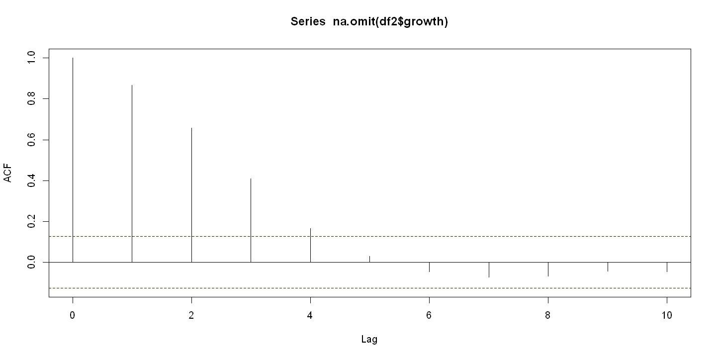
Autocorrelation
acf(na.omit(df2$growth), lag.max = 10)
12.3. 12.2 Prediction#
# Basic regression and CI at `size = 2000`
model_simple <- lm(price ~ size, data = df)
# Predict conditional mean at size = 2000
predict(model_simple, newdata = data.frame(size = 2000), interval = "confidence")
| fit | lwr | upr | |
|---|---|---|---|
| 1 | 262559.4 | 253192.2 | 271926.6 |
# Predict actual value at size = 2000
predict(model_simple, newdata = data.frame(size = 2000), interval = "prediction")
| fit | lwr | upr | |
|---|---|---|---|
| 1 | 262559.4 | 213337.9 | 311780.9 |
12.3.1. Confidence intervals manually#
xbar <- mean(df$size)
n <- nrow(df)
var_x <- var(df$size)
model <- lm(price ~ size, data = df)
b <- coef(model)
se <- summary(model)$sigma

y_cm <- b[1] + b[2]*2000
s_y_cm <- se * sqrt(1/n + (2000 - xbar)^2 / ((n - 1)*var_x))
s_y_f <- se * sqrt(1 + 1/n + (2000 - xbar)^2 / ((n - 1)*var_x))
tcrit <- qt(0.975, df = n - 2)

cat("Conditional mean CI: (", y_cm - tcrit*s_y_cm, ",", y_cm + tcrit*s_y_cm, ")\n")
cat("Prediction CI: (", y_cm - tcrit*s_y_f, ",", y_cm + tcrit*s_y_f, ")\n")
Conditional mean CI: ( 253192.2 , 271926.6 )
Prediction CI: ( 213337.9 , 311780.9 )
12.3.2. Multiple regression + CI#
model_full <- lm(price ~ size + bedrooms + bathrooms + lotsize + age + monthsold, data = df)

# Predict value for specified inputs
newdata <- data.frame(size = 2000, bedrooms = 4, bathrooms = 2, lotsize = 2, age = 40, monthsold = 6)
predict(model_full, newdata = newdata, interval = "confidence")
predict(model_full, newdata = newdata, interval = "prediction")

# Define values for predictors
new_x <- c(1, 2000, 4, 2, 2, 40, 6)  # intercept + values for size, bedrooms, etc.

# Extract coefficients and covariance matrix
beta_hat <- coef(model_full)
vcov_mat <- vcov(model_full)

# Compute point estimate (ŷ)
y_hat <- sum(new_x * beta_hat)

# Compute standard error using delta method
se_hat <- sqrt(t(new_x) %*% vcov_mat %*% new_x)

# Compute confidence interval (95%)
t_crit <- qt(0.975, df = df.residual(model_full))
ci_lower <- y_hat - t_crit * se_hat
ci_upper <- y_hat + t_crit * se_hat

# Display result
cat(sprintf("Prediction: %.2f\n", y_hat))
cat(sprintf("95%% CI: (%.2f, %.2f)\n", ci_lower, ci_upper))
| fit | lwr | upr | |
|---|---|---|---|
| 1 | 257690.8 | 244235 | 271146.6 |
| fit | lwr | upr | |
|---|---|---|---|
| 1 | 257690.8 | 204255.3 | 311126.3 |
Prediction: 257690.80
95% CI: (244234.97, 271146.63)
12.3.3. Robust SE with lincom#
Robust SE
coeftest(model_full, vcov = vcovHC(model_full, type = "HC1"))
t test of coefficients:

              Estimate Std. Error t value  Pr(>|t|)
(Intercept) 137791.066  65545.225  2.1022 0.0472030 *
size            68.369     15.359  4.4514 0.0002003 ***
bedrooms      2685.315   8285.528  0.3241 0.7489257
bathrooms     6832.880  19283.791  0.3543 0.7264632
lotsize       2303.221   5328.860  0.4322 0.6697909
age           -833.039    762.930 -1.0919 0.2866932
monthsold    -2088.504   3738.270 -0.5587 0.5820214
---
Signif. codes:  0 '***' 0.001 '**' 0.01 '*' 0.05 '.' 0.1 ' ' 1
12.4. 12.8 Bayesian Methods (Overview)#
Bayesian Regression (Informative and non-informative priors)
df$pricenew <- df$price / 1000
set.seed(10101)

# Run Bayesian regression with a valid prior ("ridge")
model_bayes <- bayesreg(pricenew ~ size, data = df, model = "normal", prior = "ridge")

summary(model_bayes)
==========================================================================================
|                   Bayesian Penalised Regression Estimation ver. 1.3                    |
|                     (c) Enes Makalic, Daniel F Schmidt. 2016-2024                      |
==========================================================================================
Bayesian Gaussian ridge regression                              Number of obs   =       29
                                                                Number of vars  =        1
MCMC Samples   =   1000                                         std(Error)      =   24.993
MCMC Burnin    =   1000                                         R-squared       =   0.6159
MCMC Thinning  =      5                                         WAIC            =   134.46

-------------+-----------------------------------------------------------------------------
   Parameter |  mean(Coef)  std(Coef)    [95% Cred. Interval]      tStat    Rank        ESS
-------------+-----------------------------------------------------------------------------
        size |     0.07007    0.01253      0.04524    0.09465      5.591       1 **     879
 (Intercept) |   121.78160   24.01663     74.02427  170.98904          .       .          .
-------------+-----------------------------------------------------------------------------