5. CHAPTER 5. BIVARIATE DATA SUMMARY#
SET UP
library(foreign) # to open stata.dta files
library(psych) # for better sammary of descriptive statistics
library(repr) # to combine graphs with adjustable plot dimensions
options(repr.plot.width = 12, repr.plot.height = 6) # Plot dimensions (in inches)
options(width = 150) # To increase character width of printed output
5.1. 5.1 EXAMPLE: HOUSE PRICE AND SIZE#
rm(list=ls())
df = read.dta(file = "Dataset/AED_HOUSE.DTA")
attach(df)
print(describe(df))
          vars  n      mean       sd median   trimmed      mad    min    max  range  skew kurtosis      se
price        1 29 253910.34 37390.71 244000 249296.00 22239.00 204000 375000 171000  1.48     2.23 6943.28
size         2 29   1882.76   398.27   1800   1836.00   296.52   1400   3300   1900  1.64     3.29   73.96
bedrooms     3 29      3.79     0.68      4      3.72     0.00      3      6      3  0.92     1.89    0.13
bathrooms    4 29      2.21     0.34      2      2.16     0.00      2      3      1  1.28     0.23    0.06
lotsize      5 29      2.14     0.69      2      2.16     0.00      1      3      2 -0.17    -1.00    0.13
age          6 29     36.41     7.12     35     36.20     5.93     23     51     28  0.44    -0.75    1.32
monthsold    7 29      5.97     1.68      6      6.04     1.48      3      8      5 -0.47    -1.03    0.31
list         8 29 257824.14 40860.26 245000 252364.00 23721.60 199900 386000 186100  1.65     2.70 7587.56
5.1.1. Table 5.1#
# price and size for sample of 29 houses
sampled_data <- df[sample(nrow(df), 29), c("price", "size")]
print(sampled_data)
    price size
10 235000 1600
26 279900 2000
29 375000 3300
23 272000 1800
15 244000 2000
19 255000 1500
22 270000 2000
11 236500 1600
1  204000 1400
7  230000 2100
14 241000 1600
28 340000 2400
8  233000 1700
18 253000 2100
20 258500 1600
12 238000 1900
3  213000 1800
24 273000 1900
9  235000 1700
16 245000 1400
2  212000 1600
5  224500 2100
6  229000 1700
27 310000 2300
21 270000 1800
4  220000 1600
17 249000 1900
25 278500 2600
13 239500 1600
5.1.2. Table 5.2#
summary(price)
quantile(price)
mean(price)
   Min. 1st Qu.  Median    Mean 3rd Qu.    Max.
 204000  233000  244000  253910  270000  375000
- 0%
- 204000
- 25%
- 233000
- 50%
- 244000
- 75%
- 270000
- 100%
- 375000
253910.344827586
summary(size)
quantile(size)
mean(size)
   Min. 1st Qu.  Median    Mean 3rd Qu.    Max.
   1400    1600    1800    1883    2000    3300
- 0%
- 1400
- 25%
- 1600
- 50%
- 1800
- 75%
- 2000
- 100%
- 3300
1882.75862068966
5.2. 5.2 TWO-WAY TABULATION#
# Create categorical variables
pricerange = price
pricerange = ifelse(price<249999, 1, 2)

sizerange = size
for (i in 1:length(sizerange)) {
    if (size[i] >= 2400) {
        sizerange[i] = 3
    }
    else if ((size[i] >= 1800)&(size[i] <= 2399)) {
        sizerange[i] = 2
    }
    else {
        sizerange[i] = 1
    }
}
5.2.1. Table 5.3#
table(pricerange,sizerange)
          sizerange
pricerange  1  2  3
         1 11  6  0
         2  2  7  3
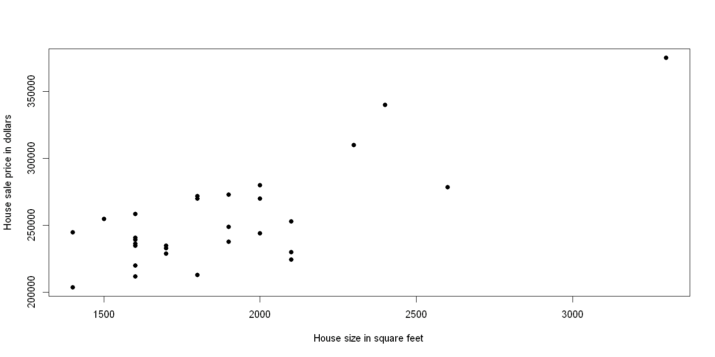
5.3. 5.3 TWOWAY SCATTER PLOT#
# Figure 5.1 First panel
plot(size, price, xlab="House size in square feet", ylab="House sale price in dollars", pch=19)
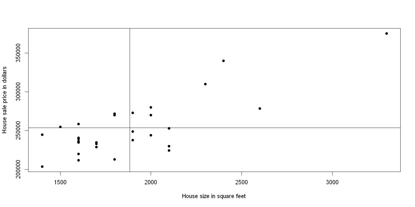
5.4. 5.4 CORRELATION#
# Figure 5.1 Second panel
plot(size, price, xlab="House size in square feet", ylab="House sale price in dollars", pch=19)
abline(253910, 0)
abline(v = 1883)
# Covariance
cov(df[,1:2])
cov(price,size)
| price | size | |
|---|---|---|
| price | 1398065246 | 11701613.3 |
| size | 11701613 | 158620.7 |
11701613.3004926
# Correlation coefficient
cor(df[,1:2])
| price | size | |
|---|---|---|
| price | 1.0000000 | 0.7857821 |
| size | 0.7857821 | 1.0000000 |
5.4.1. Plot of four cases of correlation using generated data#
# Clear the workspace
rm(list=ls())

# Set the seed number
set.seed(12345)

# Generate random data
x = rnorm(30,3,1)
u1 = rnorm(30,0,0.8)
y1 = 3 + x +u1
u2 = rnorm(30,0,2)
y2 = 3 + x + u2
y3 = 5 + u2
y4 = 10 - x - u2

cor(cbind(x,y1,y2,y3,y4))
| x | y1 | y2 | y3 | y4 | |
|---|---|---|---|---|---|
| x | 1.00000000 | 0.69802331 | 0.4175409 | 0.02760162 | -0.4175409 |
| y1 | 0.69802331 | 1.00000000 | 0.3011851 | 0.02997258 | -0.3011851 |
| y2 | 0.41754087 | 0.30118506 | 1.0000000 | 0.91983675 | -1.0000000 |
| y3 | 0.02760162 | 0.02997258 | 0.9198368 | 1.00000000 | -0.9198368 |
| y4 | -0.41754087 | -0.30118506 | -1.0000000 | -0.91983675 | 1.0000000 |
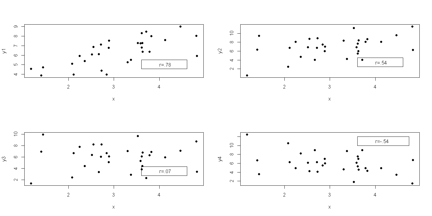
5.4.2. Figure 5.2#
par(mfrow=c(2,2))

plot(x,y1,pch=19)
legend(3.6,5.5, "r=.78", box.lwd=0)
plot(x,y2,pch=19)
legend(3.6,4.5, "r=.54", box.lwd=0)
plot(x,y3,pch=19)
legend(3.6,4.3, "r=.07", box.lwd=0)
plot(x,y4,pch=19)
legend(3.6,12, "r=-.54", box.lwd=0)

par(mfrow = c(1,1))
5.5. 5.5 REGRESSION#
# Return to house price data, firs Clear the workspace
rm(list=ls())

ols = lm(price~size)
summary(ols)
Call:
lm(formula = price ~ size)

Residuals:
   Min     1Q Median     3Q    Max
-45436 -16936   1949  17818  47932

Coefficients:
             Estimate Std. Error t value Pr(>|t|)
(Intercept) 115017.28   21489.36   5.352 1.18e-05 ***
size            73.77      11.17   6.601 4.41e-07 ***
---
Signif. codes:  0 '***' 0.001 '**' 0.01 '*' 0.05 '.' 0.1 ' ' 1

Residual standard error: 23550 on 27 degrees of freedom
Multiple R-squared:  0.6175,	Adjusted R-squared:  0.6033
F-statistic: 43.58 on 1 and 27 DF,  p-value: 4.409e-07
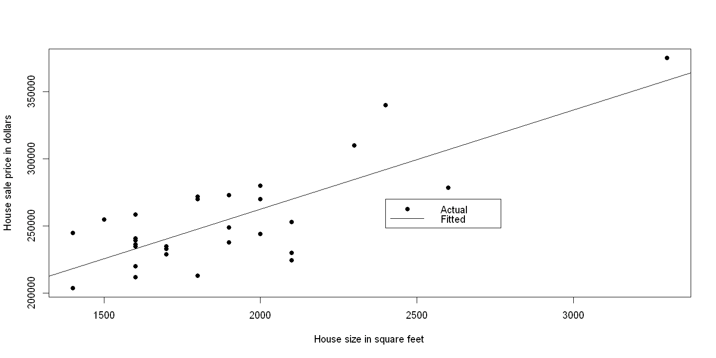
5.5.1. Figure 5.4#
plot(size,price, xlab="House size in square feet", ylab="House sale price in dollars",pch=19)
abline(ols)
legend(2400, 270000, c("Actual",  "Fitted"), lty=c(-1,1), pch=c(19,-1), bty="o")
Intercept-only regression compared to the sample mean
ols.1 = lm(price~1)
summary(ols.1)
mean(price)
Call:
lm(formula = price ~ 1)

Residuals:
   Min     1Q Median     3Q    Max
-49910 -20910  -9910  16090 121090

Coefficients:
            Estimate Std. Error t value Pr(>|t|)
(Intercept)   253910       6943   36.57   <2e-16 ***
---
Signif. codes:  0 '***' 0.001 '**' 0.01 '*' 0.05 '.' 0.1 ' ' 1

Residual standard error: 37390 on 28 degrees of freedom
253910.344827586
5.6. 5.6 MEASURES OF MODEL FIT#
# Clear the workspace
rm(list=ls())

x = 1:5

# Generate random data
set.seed(123456)
epsilon = rnorm(5,0,2)
y = 1 + 2*x + epsilon
cbind(x, epsilon, y)
summary(y)
ols.2 = lm(y~x)
summary(ols.2)
py = predict(ols.2)
resid = y - py    # ALTERNATIVELY resid = resid(ols.2)
cbind(x, epsilon, y, py, resid)
| x | epsilon | y |
|---|---|---|
| 1 | 1.6674663 | 4.667466 |
| 2 | -0.5520955 | 4.447904 |
| 3 | -0.7100037 | 6.289996 |
| 4 | 0.1749748 | 9.174975 |
| 5 | 4.5045115 | 15.504511 |
   Min. 1st Qu.  Median    Mean 3rd Qu.    Max.
  4.448   4.667   6.290   8.017   9.175  15.505
Call:
lm(formula = y ~ x)

Residuals:
     1      2      3      4      5
 1.931 -0.929 -1.727 -1.482  2.207

Coefficients:
            Estimate Std. Error t value Pr(>|t|)
(Intercept)  0.09662    2.31705   0.042   0.9694
x            2.64012    0.69862   3.779   0.0325 *
---
Signif. codes:  0 '***' 0.001 '**' 0.01 '*' 0.05 '.' 0.1 ' ' 1

Residual standard error: 2.209 on 3 degrees of freedom
Multiple R-squared:  0.8264,	Adjusted R-squared:  0.7685
F-statistic: 14.28 on 1 and 3 DF,  p-value: 0.03246
| x | epsilon | y | py | resid | |
|---|---|---|---|---|---|
| 1 | 1 | 1.6674663 | 4.667466 | 2.736739 | 1.9307278 |
| 2 | 2 | -0.5520955 | 4.447904 | 5.376855 | -0.9289502 |
| 3 | 3 | -0.7100037 | 6.289996 | 8.016971 | -1.7269744 |
| 4 | 4 | 0.1749748 | 9.174975 | 10.657087 | -1.4821119 |
| 5 | 5 | 4.5045115 | 15.504511 | 13.297203 | 2.2073086 |
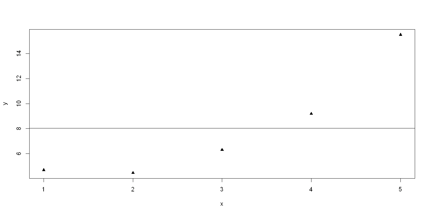
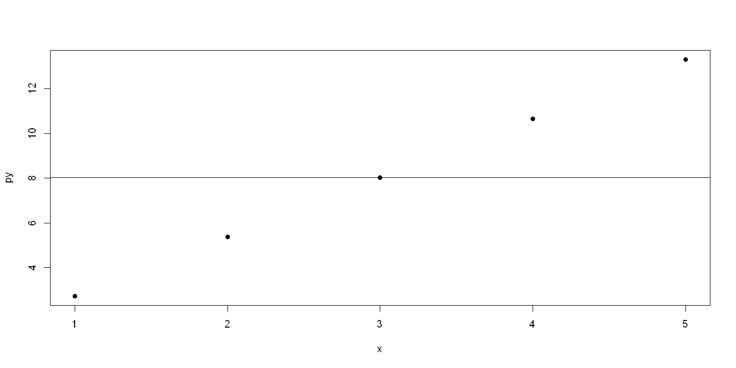
5.6.1. Figure 5.5 - Panels A and B#
plot(x,y,pch=17)
abline(8.017, 0) # The average of y is 8.017
plot(x,py,pch=19)
abline(8.017, 0) # The average of y is 8.017
5.7. 5.8 PREDICTION AND OUTLYING OBSERVATIONS#
rm(list=ls())
# df = "Dataset/AED_HOUSE.DTA")

summary(ols <- lm(price~size))
Call:
lm(formula = price ~ size)

Residuals:
   Min     1Q Median     3Q    Max
-45436 -16936   1949  17818  47932

Coefficients:
             Estimate Std. Error t value Pr(>|t|)
(Intercept) 115017.28   21489.36   5.352 1.18e-05 ***
size            73.77      11.17   6.601 4.41e-07 ***
---
Signif. codes:  0 '***' 0.001 '**' 0.01 '*' 0.05 '.' 0.1 ' ' 1

Residual standard error: 23550 on 27 degrees of freedom
Multiple R-squared:  0.6175,	Adjusted R-squared:  0.6033
F-statistic: 43.58 on 1 and 27 DF,  p-value: 4.409e-07
predict(ols, data.frame(size = 2000))
1: 262559.363354037
5.8. 5.10 CAUSATION#
# Reverse regression
reverse = lm(size~price)
summary(reverse)
Call:
lm(formula = size ~ price)

Residuals:
    Min      1Q  Median      3Q     Max
-408.18 -162.15  -24.48  150.41  511.43

Coefficients:
              Estimate Std. Error t value Pr(>|t|)
(Intercept) -2.424e+02  3.253e+02  -0.745    0.463
price        8.370e-03  1.268e-03   6.601 4.41e-07 ***
---
Signif. codes:  0 '***' 0.001 '**' 0.01 '*' 0.05 '.' 0.1 ' ' 1

Residual standard error: 250.9 on 27 degrees of freedom
Multiple R-squared:  0.6175,	Adjusted R-squared:  0.6033
F-statistic: 43.58 on 1 and 27 DF,  p-value: 4.409e-07
5.9. 5.11 COMPUTATIONs FOR CORRELATION AND REGRESSION#
# Create artificial data
rm(list=ls())
x = 1:5
y = c(1,2,2,2,3)
#cbind(x,y)

ols.3 = lm(y~x)
summary(ols.3)

cor(cbind(x,y)[,1:2])     # NOTE: SLIGHTLY DIFFERENT NUMBERS HERE
cor(x,y)^2
Call:
lm(formula = y ~ x)

Residuals:
         1          2          3          4          5
-2.000e-01  4.000e-01 -1.457e-16 -4.000e-01  2.000e-01

Coefficients:
            Estimate Std. Error t value Pr(>|t|)
(Intercept)   0.8000     0.3830   2.089   0.1279
x             0.4000     0.1155   3.464   0.0405 *
---
Signif. codes:  0 '***' 0.001 '**' 0.01 '*' 0.05 '.' 0.1 ' ' 1

Residual standard error: 0.3651 on 3 degrees of freedom
Multiple R-squared:    0.8,	Adjusted R-squared:  0.7333
F-statistic:    12 on 1 and 3 DF,  p-value: 0.04052
| x | y | |
|---|---|---|
| x | 1.0000000 | 0.8944272 |
| y | 0.8944272 | 1.0000000 |
0.8
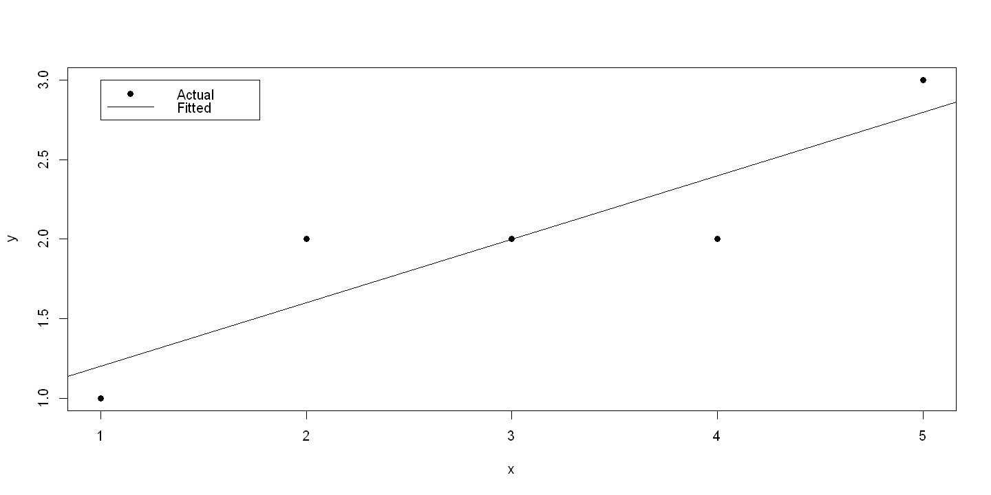
5.9.1. Figure 5.5#
plot(x,y, xlab="x", ylab="y", pch=19)
abline(ols.3)
legend(1.0, 3.0, c("Actual",  "Fitted"), lty=c(-1,1), pch=c(19,-1), bty="o")
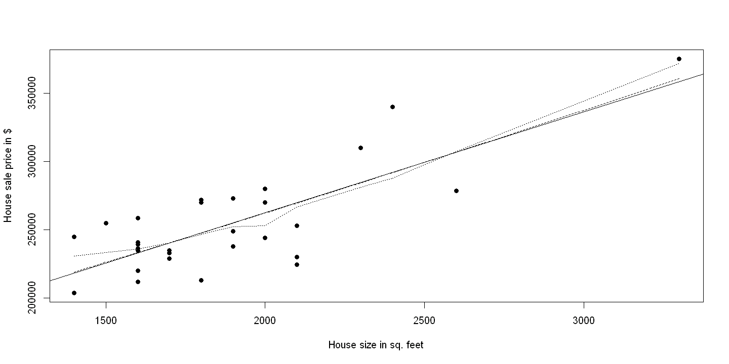
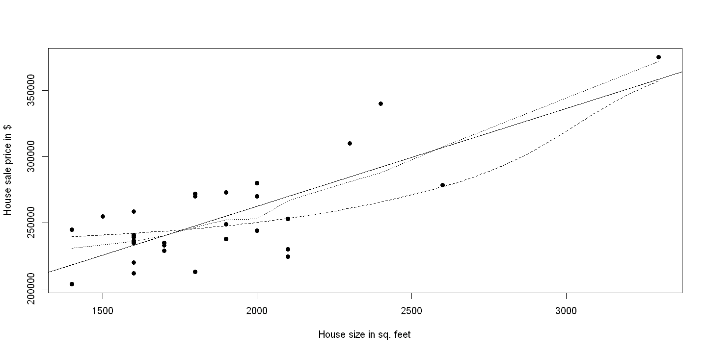
5.10. 5.12 NONPARAMETRIC REGRESSION#
summary(ols <- lm(price~size))
Call:
lm(formula = price ~ size)

Residuals:
   Min     1Q Median     3Q    Max
-45436 -16936   1949  17818  47932

Coefficients:
             Estimate Std. Error t value Pr(>|t|)
(Intercept) 115017.28   21489.36   5.352 1.18e-05 ***
size            73.77      11.17   6.601 4.41e-07 ***
---
Signif. codes:  0 '***' 0.001 '**' 0.01 '*' 0.05 '.' 0.1 ' ' 1

Residual standard error: 23550 on 27 degrees of freedom
Multiple R-squared:  0.6175,	Adjusted R-squared:  0.6033
F-statistic: 43.58 on 1 and 27 DF,  p-value: 4.409e-07
plot(size,price, xlab="House size in sq. feet", ylab="House sale price in $",pch=19)
abline(ols)
lines(lowess(size,price), lty=3)
lines(ksmooth(size,price, "normal", bandwidth = 1000), lty=2)
# For local linear use kernsmooth package and locpoly command
suppressPackageStartupMessages(library(KernSmooth))
plot(size,price, xlab="House size in sq. feet", ylab="House sale price in $",pch=19)
abline(ols)
lines(lowess(size,price), lty=3)
lines(locpoly(size, price, bandwidth = 2000, kernel=epan), lty=2)