6. CHAPTER 6. THE LEAST SQUARE ESTIMATOR#
SET UP
library(foreign) # to open stata.dta files
library(psych) # for better sammary of descriptive statistics
library(repr) # to combine graphs with adjustable plot dimensions
options(repr.plot.width = 12, repr.plot.height = 6) # Plot dimensions (in inches)
options(width = 150) # To increase character width of printed output
6.1. 6.2 EXAMPLES OF SAMPLING FROM A POPULATION#
rm(list=ls())
df = read.dta(file = "Dataset/AED_GENERATEDDATA.DTA")
attach(df)
df_desc<-describe(df)
print(df_desc)
         vars n  mean   sd median trimmed  mad   min   max range skew kurtosis   se
x           1 5  3.00 1.58   3.00    3.00 1.48  1.00  5.00  4.00 0.00    -1.91 0.71
Eygivenx    2 5  7.00 3.16   7.00    7.00 2.97  3.00 11.00  8.00 0.00    -1.91 1.41
u           3 5 -1.03 1.75  -1.63   -1.03 1.29 -2.51  1.69  4.20 0.54    -1.66 0.78
y           4 5  5.97 1.90   4.69    5.97 0.29  4.49  8.61  4.12 0.40    -2.03 0.85
6.1.1. Table 6.1#
print(df.head<-head(df))
  x Eygivenx          u        y
1 1        3  1.6898891 4.689889
2 2        5 -0.3187171 4.681283
3 3        7 -2.5066674 4.493333
4 4        9 -1.6332803 7.366720
5 5       11 -2.3907640 8.609236
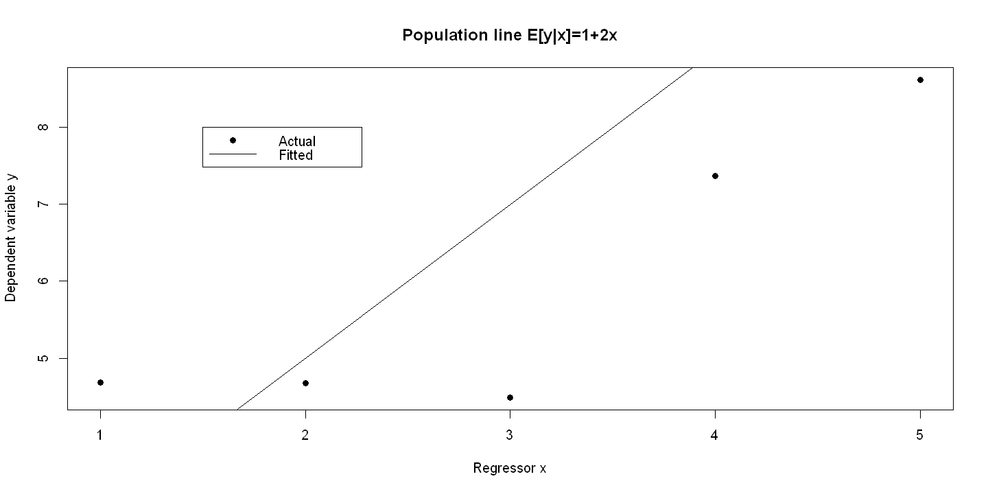
6.1.2. Figure 6.2: panel A#
summary(olsEyx <- lm(Eygivenx ~ x))

plot(x, y, xlab="Regressor x", ylab="Dependent variable y", pch=19, main="Population line E[y|x]=1+2x")
abline(olsEyx)
legend(1.5, 8, c("Actual",  "Fitted"), lty=c(-1,1), pch=c(19,-1), bty="o")
Warning message in summary.lm(olsEyx <- lm(Eygivenx ~ x)):
"essentially perfect fit: summary may be unreliable"
Call:
lm(formula = Eygivenx ~ x)

Residuals:
         1          2          3          4          5
 7.134e-19  6.054e-16 -7.714e-16 -2.760e-16  4.414e-16

Coefficients:
             Estimate Std. Error   t value Pr(>|t|)
(Intercept) 1.000e+00  6.723e-16 1.487e+15   <2e-16 ***
x           2.000e+00  2.027e-16 9.867e+15   <2e-16 ***
---
Signif. codes:  0 '***' 0.001 '**' 0.01 '*' 0.05 '.' 0.1 ' ' 1

Residual standard error: 6.41e-16 on 3 degrees of freedom
Multiple R-squared:      1,	Adjusted R-squared:      1
F-statistic: 9.736e+31 on 1 and 3 DF,  p-value: < 2.2e-16
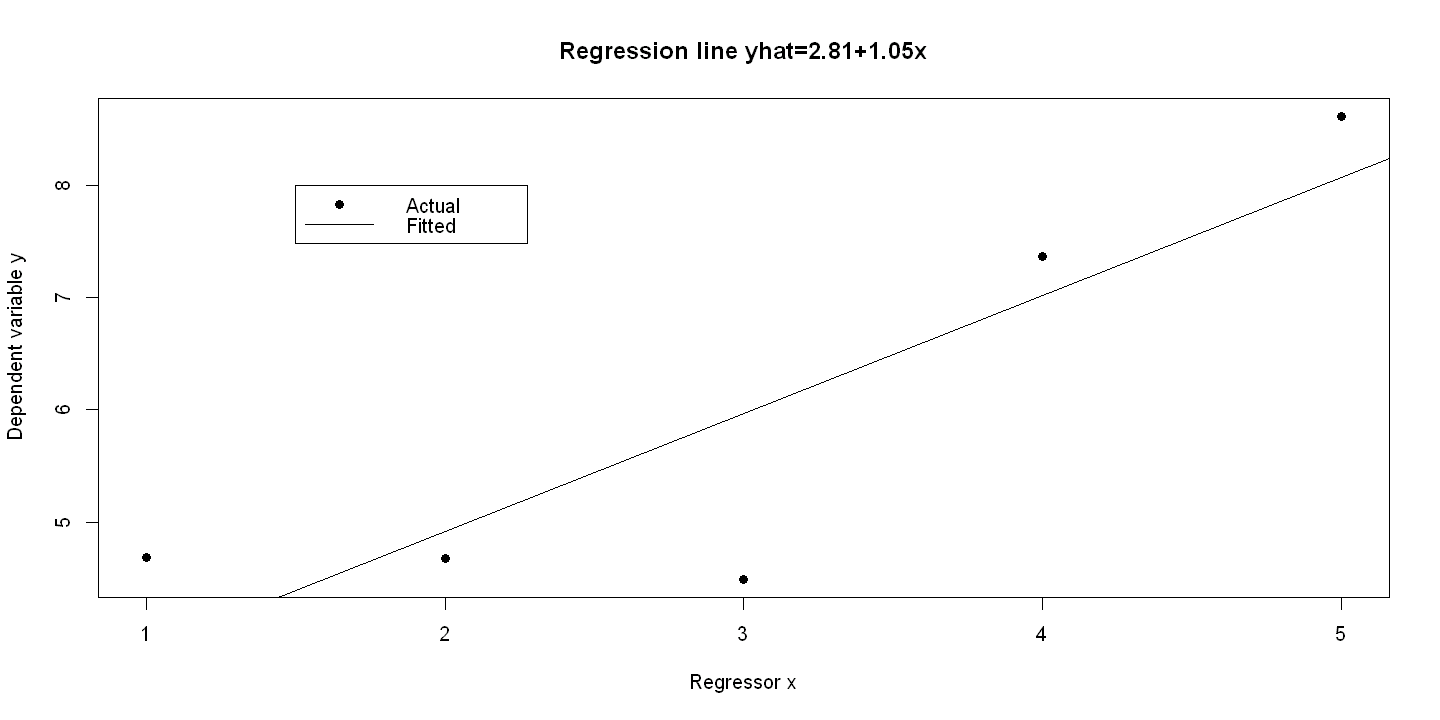
6.1.3. Figure 6.2: panel B#
olsyx <- lm(y ~ x)
summary(olsyx)
plot(x, y, xlab="Regressor x", ylab="Dependent variable y",pch=19, main = "Regression line yhat=2.81+1.05x" )
abline(olsyx)
legend(1.5, 8, c("Actual",  "Fitted"), lty=c(-1,1), pch=c(19,-1), bty="o")
Call:
lm(formula = y ~ x)

Residuals:
      1       2       3       4       5
 0.8266 -0.2344 -1.4748  0.3462  0.5363

Coefficients:
            Estimate Std. Error t value Pr(>|t|)
(Intercept)   2.8109     1.1034   2.547   0.0841 .
x             1.0524     0.3327   3.163   0.0507 .
---
Signif. codes:  0 '***' 0.001 '**' 0.01 '*' 0.05 '.' 0.1 ' ' 1

Residual standard error: 1.052 on 3 degrees of freedom
Multiple R-squared:  0.7693,	Adjusted R-squared:  0.6925
F-statistic: 10.01 on 1 and 3 DF,  p-value: 0.05074
Three regressions from the same model
rm(list=ls())
set.seed(12345)
u = runif(30,min=0,max=1)
x1 = rnorm(30,3,1)
u1 = rnorm(30,0,2)
y1 = 1 + 2*x1 + u1
x2 = rnorm(30,3,1)
u2 = rnorm(30,0,2)
y2 = 1 + 2*x2 + u2
x3 = rnorm(30,3,1)
u3 = rnorm(30,0,2)
y3 = 1 + 2*x3 + u3
ols1 <- lm(y1 ~ x1)
summary(ols1)
ols2 <- lm(y2 ~ x2)
summary(ols2)
ols3 <- lm(y3 ~ x3)
summary(ols3)
Call:
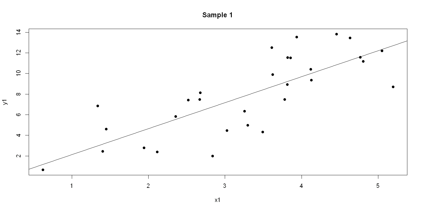
lm(formula = y1 ~ x1)
Residuals:
Min 1Q Median 3Q Max
-4.783 -1.612 -0.090 1.693 4.003
Coefficients:
Estimate Std. Error t value Pr(>|t|)
(Intercept) -0.3789 1.3276 -0.285 0.777
x1 2.5173 0.3806 6.614 3.56e-07 ***
---
Signif. codes: 0 '***' 0.001 '**' 0.01 '*' 0.05 '.' 0.1 ' ' 1
Residual standard error: 2.442 on 28 degrees of freedom
Multiple R-squared: 0.6097, Adjusted R-squared: 0.5958
F-statistic: 43.75 on 1 and 28 DF, p-value: 3.565e-07
Call:
lm(formula = y2 ~ x2)

Residuals:
   Min     1Q Median     3Q    Max
-4.623 -1.528 -0.207  2.122  4.896

Coefficients:
            Estimate Std. Error t value Pr(>|t|)
(Intercept)   1.2469     1.5805   0.789 0.436775
x2            2.0538     0.4584   4.480 0.000115 ***
---
Signif. codes:  0 '***' 0.001 '**' 0.01 '*' 0.05 '.' 0.1 ' ' 1

Residual standard error: 2.528 on 28 degrees of freedom
Multiple R-squared:  0.4176,	Adjusted R-squared:  0.3968
F-statistic: 20.07 on 1 and 28 DF,  p-value: 0.0001146
Call:
lm(formula = y3 ~ x3)

Residuals:
    Min      1Q  Median      3Q     Max
-3.9398 -0.9904  0.1098  1.0261  3.8738

Coefficients:
            Estimate Std. Error t value Pr(>|t|)
(Intercept)   2.7696     1.2548   2.207  0.03567 *
x3            1.5345     0.4433   3.461  0.00174 **
---
Signif. codes:  0 '***' 0.001 '**' 0.01 '*' 0.05 '.' 0.1 ' ' 1

Residual standard error: 1.927 on 28 degrees of freedom
Multiple R-squared:  0.2997,	Adjusted R-squared:  0.2747
F-statistic: 11.98 on 1 and 28 DF,  p-value: 0.001742
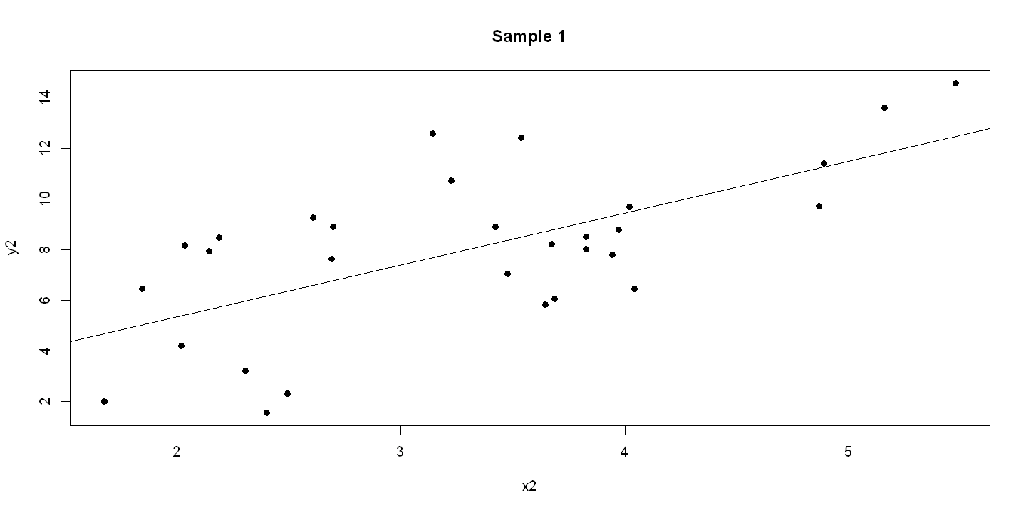
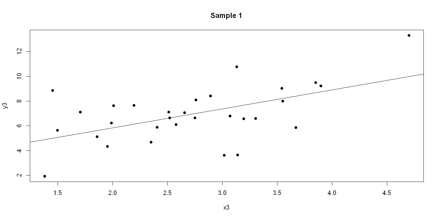
6.1.4. Figure 6.3 - three panels#
plot(x1, y1, pch=19, main = "Sample 1" )
abline(ols1)
plot(x2, y2, pch=19, main = "Sample 1" )
abline(ols2)
plot(x3, y3, pch=19, main = "Sample 1" )
abline(ols3)
Generated data: results of regression on 400 samples of size 30
df = read.dta(file = "Dataset/AED_GENERATEDREGRESSIONS.DTA")
attach(df)
df_desc<-describe(df)
print(df_desc)
head(df)
            vars   n  mean   sd median trimmed  mad   min   max range  skew kurtosis   se
slope          1 400  1.99 0.38   1.96    1.98 0.38  0.59  3.17  2.58  0.04     0.19 0.02
seslope        2 400  0.38 0.07   0.37    0.37 0.07  0.19  0.65  0.46  0.60     0.42 0.00
intercept      3 400  1.02 1.19   1.06    1.03 1.13 -2.46  5.67  8.13 -0.05     0.16 0.06
seintercept    4 400  1.19 0.23   1.17    1.18 0.22  0.63  2.00  1.37  0.60     0.47 0.01
rsquared       5 400  0.50 0.12   0.51    0.50 0.12  0.09  0.82  0.73 -0.40     0.17 0.01
numobs         6 400 30.00 0.00  30.00   30.00 0.00 30.00 30.00  0.00   NaN      NaN 0.00
| slope | seslope | intercept | seintercept | rsquared | numobs | |
|---|---|---|---|---|---|---|
| <dbl> | <dbl> | <dbl> | <dbl> | <dbl> | <dbl> | |
| 1 | 2.011422 | 0.2921605 | 0.9837164 | 0.9583587 | 0.6286392 | 30 |
| 2 | 1.634170 | 0.3506421 | 1.7954644 | 1.1950867 | 0.4368498 | 30 |
| 3 | 2.094961 | 0.4156610 | -0.0209372 | 1.3890935 | 0.4756781 | 30 |
| 4 | 1.972498 | 0.2285200 | 0.6164197 | 0.8136204 | 0.7268423 | 30 |
| 5 | 2.548882 | 0.6503775 | -0.6771045 | 1.9628325 | 0.3542315 | 30 |
| 6 | 2.064110 | 0.3353717 | 1.2542309 | 0.9950362 | 0.5749864 | 30 |
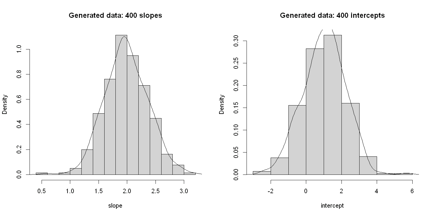
6.1.5. Figure 6.4#
par(mfrow=c(1,2))

# Panel A
hist(slope, freq=FALSE, xlab="slope", main="Generated data: 400 slopes")
lines(density(slope))

# Panel B
hist(intercept, prob=TRUE, xlab="intercept", main="Generated data: 400 intercepts")
lines(density(intercept))

par(mfrow = c(1,1))
Census data: results of regression on 400 samples of size 120
df = read.dta(file = "Dataset/AED_CENSUSREGRESSIONS.DTA")
attach(df)
df_desc<-describe(df)
print(df_desc)
head(df)
The following objects are masked from df (pos = 3):

    intercept, numobs, seintercept, seslope, slope
vars n mean sd median trimmed mad min max range skew kurtosis se
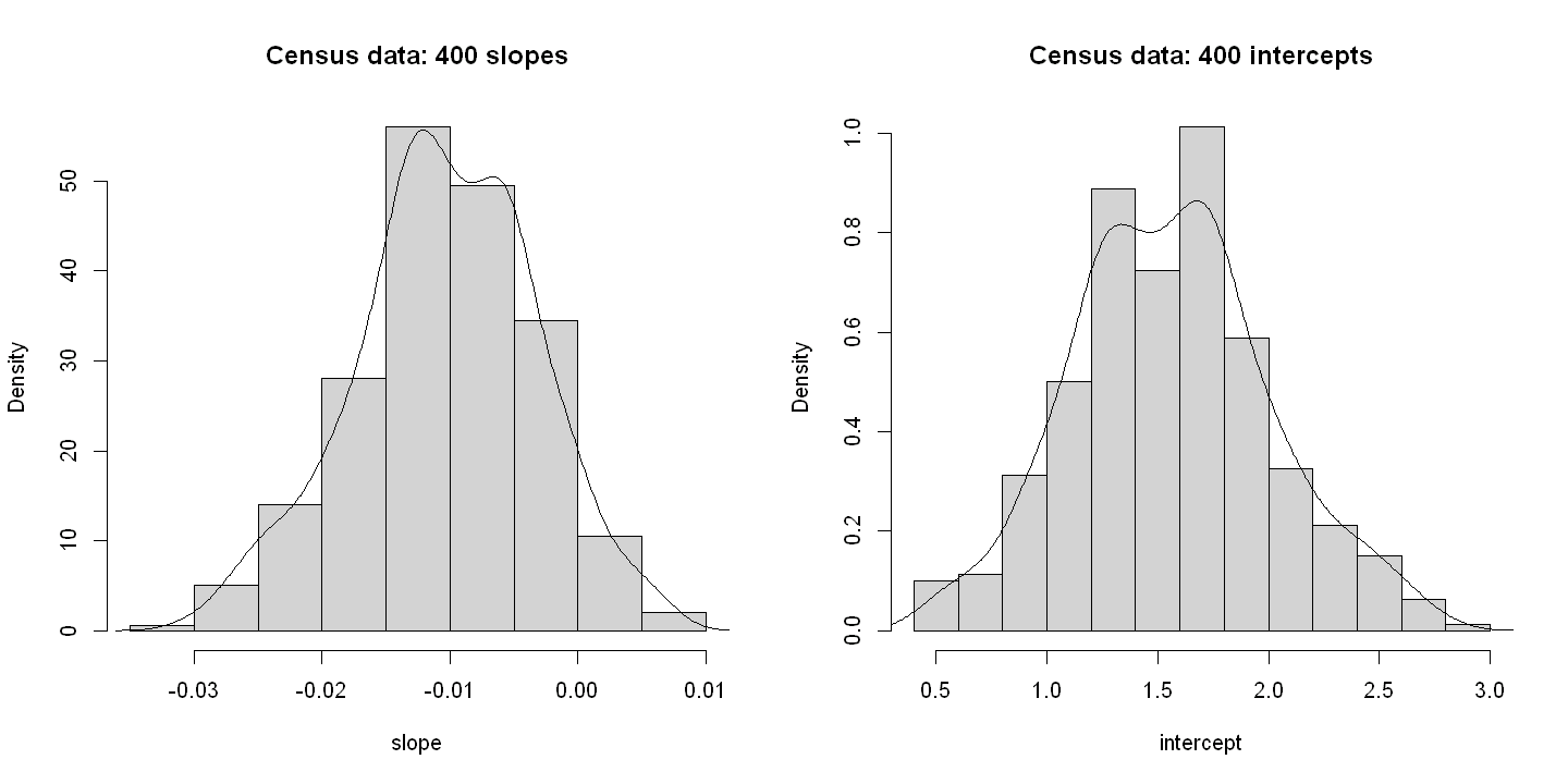
slope 1 400 -0.01 0.01 -0.01 -0.01 0.01 -0.03 0.01 0.04 -0.18 -0.15 0.00
seslope 2 400 0.01 0.00 0.01 0.01 0.00 0.00 0.01 0.00 -0.11 -0.02 0.00
intercept 3 400 1.56 0.45 1.55 1.55 0.43 0.45 2.80 2.36 0.17 -0.14 0.02
seintercept 4 400 0.41 0.04 0.42 0.41 0.04 0.31 0.53 0.23 -0.12 -0.03 0.00
numobs 5 400 200.00 0.00 200.00 200.00 0.00 200.00 200.00 0.00 NaN NaN 0.00
| slope | seslope | intercept | seintercept | numobs | |
|---|---|---|---|---|---|
| <dbl> | <dbl> | <dbl> | <dbl> | <dbl> | |
| 1 | -0.01326593 | 0.007451856 | 1.707933 | 0.4797598 | 200 |
| 2 | -0.01021786 | 0.006931265 | 1.534607 | 0.4446451 | 200 |
| 3 | -0.00404300 | 0.006063364 | 1.174318 | 0.3894077 | 200 |
| 4 | -0.01864705 | 0.005981046 | 2.090928 | 0.3841836 | 200 |
| 5 | -0.01285031 | 0.006403644 | 1.704155 | 0.4113336 | 200 |
| 6 | -0.01622651 | 0.006049114 | 1.949338 | 0.3898587 | 200 |
6.1.6. Figure 6.5#
par(mfrow = c(1,2))

# Panel A
hist(slope, freq=FALSE, xlab="slope", main="Census data: 400 slopes")
lines(density(slope))

# Panel B
hist(intercept, prob=TRUE, xlab="intercept", main="Census data: 400 intercepts")
lines(density(intercept))