3. CHAPTER 3. THE SAMPLE MEAN#
SET UP
library(foreign) # to open stata.dta files
library(psych) # for better sammary of descriptive statistics
library(repr) # to combine graphs with adjustable plot dimensions
options(repr.plot.width = 12, repr.plot.height = 6) # Plot dimensions (in inches)
options(width = 150) # To increase character width of printed output
3.1. 3.2 SAMPLE GENERATED BY AN EXPERIMENT: COIN TOSSES#
# Draw one sample of size 30 from Bernoulli mu = p = 0.5
rm(list=ls())
set.seed(10101)
u = runif(30,min=0,max=1)
x = ifelse(u > 0.5, 1, 0)
print(describe(cbind(x,u)))
table(x)
  vars  n mean   sd median trimmed  mad  min  max range  skew kurtosis   se
x    1 30 0.60 0.50   1.00    0.62 0.00 0.00 1.00  1.00 -0.39    -1.91 0.09
u    2 30 0.52 0.31   0.57    0.52 0.37 0.02 0.98  0.95 -0.17    -1.39 0.06
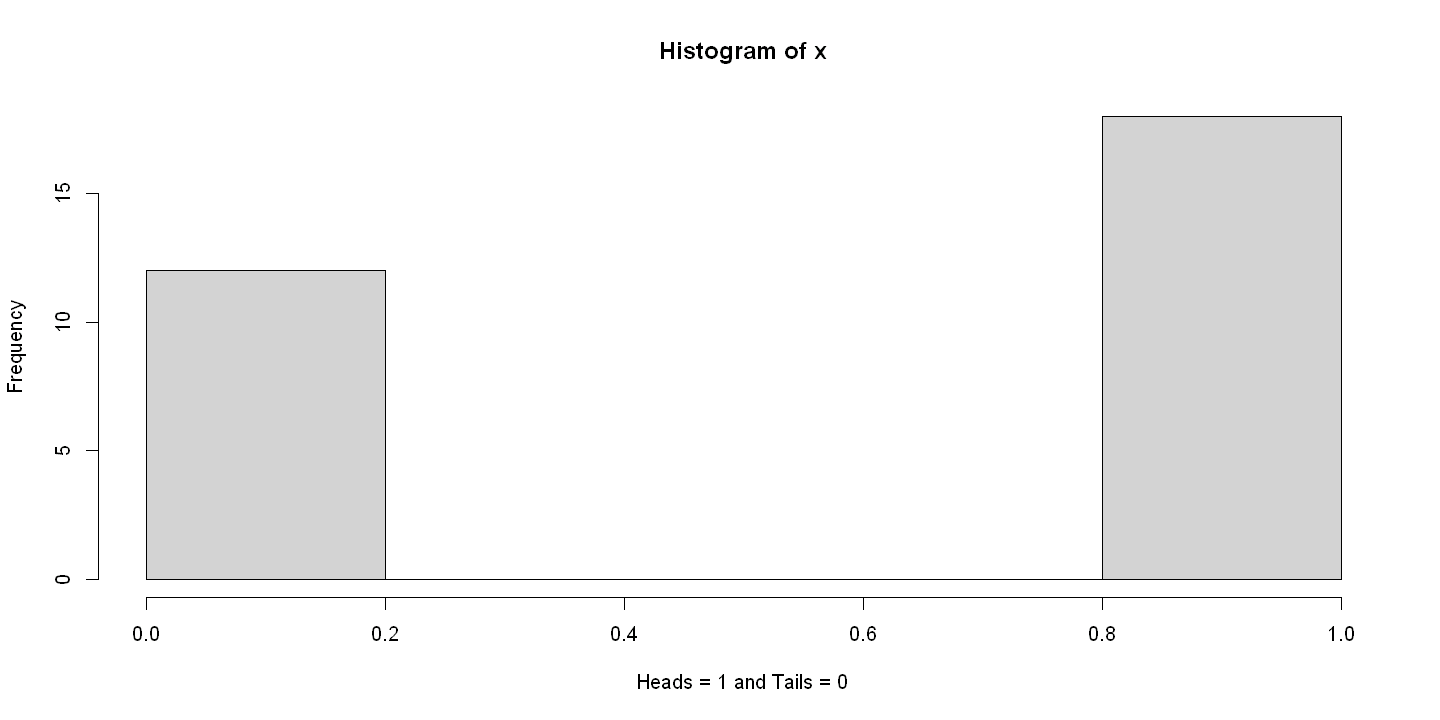
x
 0  1
12 18
3.2. Figure 3.1: First panel#
hist(x,xlab="Heads = 1 and Tails = 0")
rm(list=ls())
df = read.dta(file = "Dataset/AED_COINTOSSMEANS.DTA") # Data for 400 coin tosses
attach(df)
# Summarize the data set
print((describe(df)))
print(head(df, n=5))
       vars   n mean   sd median trimmed  mad   min   max range  skew kurtosis se
xbar      1 400  0.5 0.09    0.5     0.5 0.10  0.27  0.73  0.47 -0.02    -0.27  0
stdev     2 400  0.5 0.01    0.5     0.5 0.01  0.45  0.51  0.06 -2.03     4.40  0
numobs    3 400 30.0 0.00   30.0    30.0 0.00 30.00 30.00  0.00   NaN      NaN  0
       xbar     stdev numobs
1 0.3333333 0.4794633     30
2 0.5000000 0.5085476     30
3 0.5333334 0.5074162     30
4 0.5666667 0.5040069     30
5 0.5000000 0.5085476     30
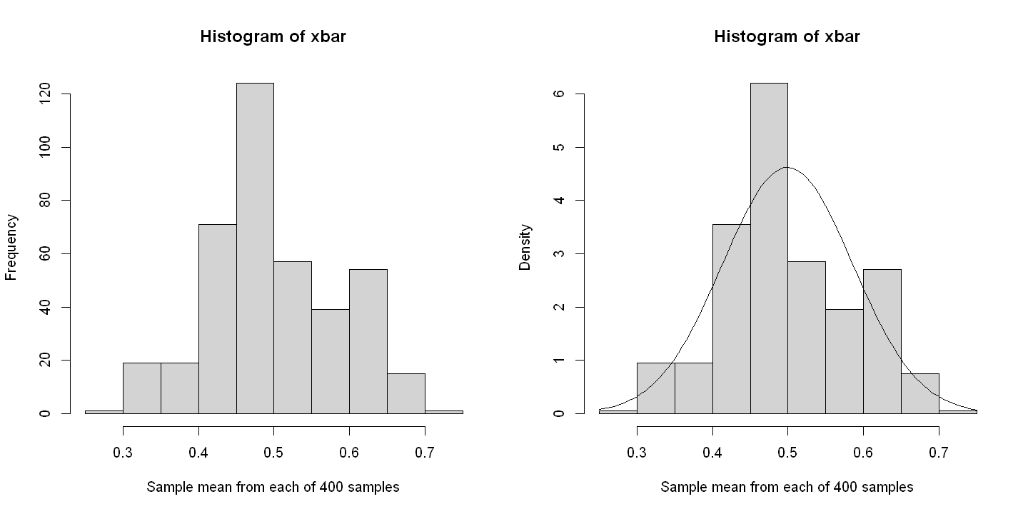
par(mfrow=c(1,2))
hist(xbar,xlab="Sample mean from each of 400 samples")
hist(xbar, xlab="Sample mean from each of 400 samples", freq=FALSE)
x<-seq(0, 1, by=0.02)    # need x here and not some other name
curve(dnorm(x,mean(xbar),sd(xbar)), add=TRUE)
3.3. 3.4 SAMPLING FROM A FINITE POPULATION: 1880 U.S. CENSUS#
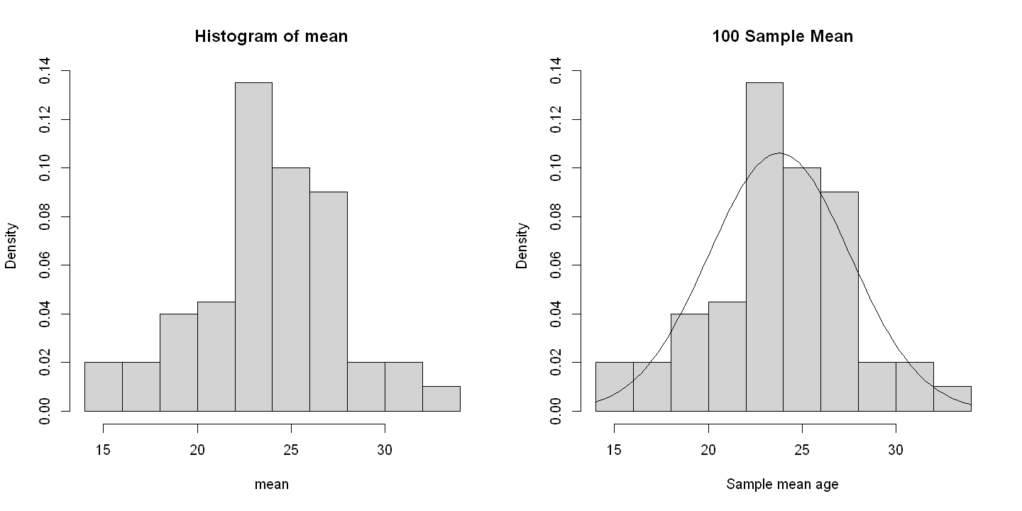
3.3.1. Figure 3.3#
# Means from 100 samples of size 25
rm(list=ls())
df.age = read.dta(file = "Dataset/AED_CENSUSAGEMEANS.DTA")
print((describe(df.age)))
       vars   n  mean   sd median trimmed  mad   min   max range  skew kurtosis   se
mean      1 100 23.78 3.76  23.76   23.85 3.35 14.60 33.44 18.84 -0.13     0.14 0.38
stdev     2 100 18.25 2.89  18.43   18.29 3.08 12.36 25.31 12.94 -0.11    -0.59 0.29
numobs    3 100 25.00 0.00  25.00   25.00 0.00 25.00 25.00  0.00   NaN      NaN 0.00
print(head(df.age, n=5))
   mean    stdev numobs
1 27.84 20.70765     25
2 19.40 16.00000     25
3 23.28 19.02087     25
4 26.84 20.50951     25
5 26.56 20.19299     25
attach(df.age)
par(mfrow=c(1,2))
# Figure 3.3 second panel  Histogram for 100 means
hist(mean, freq=FALSE)

# Figure 3.2 second panel  Histogram for 100 means plus normal curve
hist(mean, main="100 Sample Mean", xlab="Sample mean age", freq=FALSE)
x<-seq(0, 50, by=0.2)
curve(dnorm(x, mean(mean), sd(mean)), add=TRUE)
The following objects are masked from df:

    numobs, stdev
3.4. 3.7 COMPUTER GENERATION OF A RANDOM SAMPLE#
# Single sample
set.seed(10101)
x=runif(100,min=3,max=9)
y=rnorm(100,5,2)

# Mean of 400 coin toss samples each of size 30
set.seed(10101)
result.mean=array(dim=400)
result.stdev=array(dim=400)
for(i in 1:400){
    x=rbinom(30,1,0.5)
    result.mean[i]=mean(x)
    result.stdev[i]=sd(x)
}
mean(result.mean)
sd(result.mean)
summary(result.mean)
0.500583333333333
0.0907728121478548
   Min. 1st Qu.  Median    Mean 3rd Qu.    Max.
 0.2667  0.4333  0.5000  0.5006  0.5667  0.7667