13. CHAPTER 13. CASE STUDIES FOR MULTIPLE REGRESSION#
SET UP
library(foreign) # to open stata.dta files
library(psych) # for better sammary of descriptive statistics
library(repr) # to combine graphs with adjustable plot dimensions
options(repr.plot.width = 12, repr.plot.height = 6) # Plot dimensions (in inches)
options(width = 150) # To increase character width of printed output
13.1. 13.1 Case Study 1: School Performance Index#
13.1.1. California Academic Performance Index#
df <- read.dta("Dataset/AED_API99.DTA")
attach(df)
df_desc<-describe(df)
print(df_desc)
           vars   n       mean         sd     median    trimmed        mad       min       max      range  skew kurtosis       se
sch_code      1 807 2878752.53 1428937.22 3033578.00 2871983.47 1629414.46 130054.00 5838305.0 5708251.00  0.02    -0.80 50300.97
api99         2 807     620.94     107.44     620.00     619.67     112.68    355.00     966.0     611.00  0.12    -0.40     3.78
edparent      3 807      12.84       1.23      12.88      12.85       1.22      9.62      16.0       6.38 -0.09    -0.33     0.04
meals         4 807      21.92      23.67      14.00      18.48      20.76      0.00      98.0      98.00  0.96    -0.06     0.83
englearn      5 807      14.00      12.79      10.00      12.24      11.86      0.00      66.0      66.00  1.17     1.06     0.45
yearround     6 807       0.02       0.15       0.00       0.00       0.00      0.00       1.0       1.00  6.27    37.40     0.01
credteach     7 807      89.84       8.44      92.00      90.80       7.41     33.00     100.0      67.00 -1.38     3.60     0.30
emerteach     8 807      10.46       8.21       9.00       9.59       7.41      0.00      56.0      56.00  1.45     3.78     0.29
avg_ed_raw    9 807       2.92       0.62       2.94       2.93       0.61      1.31       4.5       3.19 -0.09    -0.33     0.02
pct_af_am    10 807       7.24      11.11       3.00       4.83       2.97      0.00      79.0      79.00  3.26    13.45     0.39
pct_am_ind   11 807       1.15       3.21       1.00       0.64       1.48      0.00      63.0      63.00 12.60   212.38     0.11
pct_asian    12 807       9.27      12.20       5.00       6.61       5.93      0.00      70.0      70.00  2.32     5.90     0.43
pct_fil      13 807       2.59       4.68       1.00       1.58       1.48      0.00      44.0      44.00  4.62    28.86     0.16
pct_hisp     14 807      33.27      24.87      27.00      30.42      23.72      1.00      99.0      98.00  0.84    -0.23     0.88
pct_pac      15 807       0.52       0.96       0.00       0.32       0.00      0.00      10.0      10.00  3.49    20.02     0.03
pct_white    16 807      45.71      27.90      46.00      45.88      37.06      0.00      97.0      97.00 -0.04    -1.26     0.98
mobility     17 757      13.78      18.21       9.00       9.71       5.93      0.00     100.0     100.00  3.28    11.38     0.66
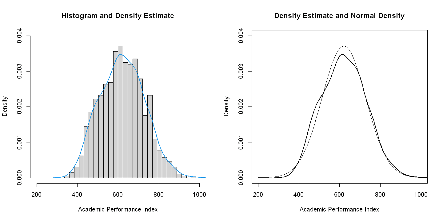
13.1.2. Univariate Analysis#
par(mfrow=c(1,2))
hist(api99, prob = TRUE, xlim=c(200,1000), ylim = c(0, 0.004),
     breaks=c(24*0:42), main="Histogram and Density Estimate", xlab="Academic Performance Index" )
lines(density(api99), col = 4, lwd = 2)
plot(density(api99), main="Density Estimate and Normal Density", xlab="Academic Performance Index",
     ylim = c(0, 0.004), xlim=c(200,1000), type="l", lwd=2)
x<-seq(0, 1, by=0.02)    # need x here and not some other name
curve(dnorm(x,mean(api99),sd(api99)), add=TRUE)
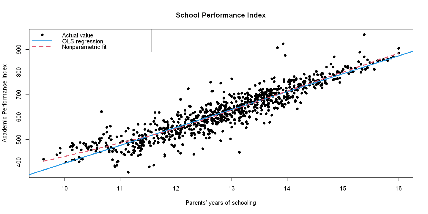
13.1.3. Bivariate Analysis#
library(jtools)
summ(ols_api<- lm(api99 ~ edparent), digits=4)
MODEL INFO:
Observations: 807
Dependent Variable: api99
Type: OLS linear regression

MODEL FIT:
F(1,805) = 4072.8500, p = 0.0000
R² = 0.8350
Adj. R² = 0.8348

Standard errors:OLS
-----------------------------------------------------------
                         Est.      S.E.     t val.        p
----------------- ----------- --------- ---------- --------
(Intercept)         -400.3137   16.0761   -24.9011   0.0000
edparent              79.5292    1.2462    63.8189   0.0000
-----------------------------------------------------------
plot(edparent, api99,
     xlab = "Parents' years of schooling",
     ylab = "Academic Performance Index",
     pch = 19,
     main = "School Performance Index")

abline(ols_api, lwd = 3, col = 4)

lines(lowess(edparent, api99), lwd = 3, lty = 2, col = 2)

legend("topleft",
       legend = c("Actual value", "OLS regression", "Nonparametric fit"),
       lty = c(NA, 1, 2),
       pch = c(19, NA, NA),
       col = c("black", 4, 2),
       lwd = c(NA, 3, 3),
       bty = "o")
13.1.4. Correlation#
print(cor(cbind(api99, edparent, meals,englearn,yearround,credteach,emerteach)))
               api99   edparent      meals   englearn   yearround  credteach   emerteach
api99      1.0000000  0.9137660 -0.5419036 -0.6561381 -0.19355145  0.4592823 -0.45331322
edparent   0.9137660  1.0000000 -0.6046625 -0.7071808 -0.24685800  0.3967105 -0.37020234
meals     -0.5419036 -0.6046625  1.0000000  0.5598149  0.29042515 -0.2729162  0.21499672
englearn  -0.6561381 -0.7071808  0.5598149  1.0000000  0.22315910 -0.2606307  0.20265116
yearround -0.1935514 -0.2468580  0.2904251  0.2231591  1.00000000 -0.1811366  0.09374574
credteach  0.4592823  0.3967105 -0.2729162 -0.2606307 -0.18113659  1.0000000 -0.81944305
emerteach -0.4533132 -0.3702023  0.2149967  0.2026512  0.09374574 -0.8194430  1.00000000
13.1.5. Multiple regression#
summ(ols_api_multi<-lm(api99~edparent + meals+englearn+yearround+credteach+emerteach), digits=3)
MODEL INFO:
Observations: 807
Dependent Variable: api99
Type: OLS linear regression

MODEL FIT:
F(6,800) = 771.411, p = 0.000
R² = 0.853
Adj. R² = 0.852

Standard errors:OLS
------------------------------------------------------
                        Est.     S.E.   t val.       p
----------------- ---------- -------- -------- -------
(Intercept)         -345.328   39.954   -8.643   0.000
edparent              73.942    1.883   39.273   0.000
meals                  0.079    0.081    0.980   0.327
englearn              -0.358    0.167   -2.145   0.032
yearround             25.956   10.185    2.548   0.011
credteach              0.387    0.311    1.247   0.213
emerteach             -1.470    0.315   -4.672   0.000
------------------------------------------------------
13.2. 13.2 Cobb-Douglas Production Function#
df <- read.dta("Dataset/AED_COBBDOUGLAS.DTA")
attach(df)
print(df)
   year   q   k   l      lnq      lnk      lnl
1  1899 100 100 100 4.605170 4.605170 4.605170
2  1900 101 107 105 4.615120 4.672829 4.653960
3  1901 112 114 110 4.718499 4.736198 4.700480
4  1902 122 122 118 4.804021 4.804021 4.770685
5  1903 124 131 123 4.820282 4.875197 4.812184
6  1904 122 138 116 4.804021 4.927254 4.753590
7  1905 143 149 125 4.962845 5.003946 4.828314
8  1906 152 163 133 5.023880 5.093750 4.890349
9  1907 151 176 138 5.017280 5.170484 4.927254
10 1908 126 185 121 4.836282 5.220356 4.795791
11 1909 155 198 140 5.043425 5.288267 4.941642
12 1910 159 208 144 5.068904 5.337538 4.969813
13 1911 153 216 145 5.030438 5.375278 4.976734
14 1912 177 226 152 5.176150 5.420535 5.023880
15 1913 184 236 154 5.214936 5.463832 5.036952
16 1914 169 244 149 5.129899 5.497168 5.003946
17 1915 189 266 154 5.241747 5.583496 5.036952
18 1916 225 298 182 5.416101 5.697093 5.204007
19 1917 227 335 196 5.424950 5.814130 5.278115
20 1918 223 366 200 5.407172 5.902633 5.298317
21 1919 218 387 193 5.384495 5.958425 5.262690
22 1920 231 407 193 5.442418 6.008813 5.262690
23 1921 179 417 147 5.187386 6.033086 4.990433
24 1922 240 431 161 5.480639 6.066108 5.081404
print(describe(df))
     vars  n    mean     sd  median trimmed    mad     min     max  range  skew kurtosis    se
year    1 24 1910.50   7.07 1910.50 1910.50   8.90 1899.00 1922.00  23.00  0.00    -1.35  1.44
q       2 24  165.92  43.75  157.00  165.50  48.18  100.00  240.00 140.00  0.21    -1.28  8.93
k       3 24  234.17 106.27  212.00  228.25 114.90  100.00  431.00 331.00  0.52    -1.13 21.69
l       4 24  145.79  29.62  144.50  144.90  30.39  100.00  200.00 100.00  0.40    -0.95  6.05
lnq     5 24    5.08   0.27    5.06    5.09   0.34    4.61    5.48   0.88 -0.12    -1.22  0.05
lnk     6 24    5.36   0.46    5.36    5.36   0.58    4.61    6.07   1.46  0.03    -1.30  0.09
lnl     7 24    4.96   0.20    4.97    4.96   0.23    4.61    5.30   0.69  0.10    -1.02  0.04
summ(ols_cd<-lm(lnq~lnk+lnl),digits=3)
MODEL INFO:
Observations: 24
Dependent Variable: lnq
Type: OLS linear regression

MODEL FIT:
F(2,21) = 236.122, p = 0.000
R² = 0.957
Adj. R² = 0.953

Standard errors:OLS
---------------------------------------------------
                      Est.    S.E.   t val.       p
----------------- -------- ------- -------- -------
(Intercept)         -0.177   0.434   -0.408   0.687
lnk                  0.233   0.064    3.668   0.001
lnl                  0.807   0.145    5.565   0.000
---------------------------------------------------
suppressPackageStartupMessages(library(car))
print(linearHypothesis(ols_cd,c("lnk=0.25","lnl=0.75")))
Linear hypothesis test:
lnk = 0.25
lnl = 0.75

Model 1: restricted model
Model 2: lnq ~ lnk + lnl

  Res.Df      RSS Df  Sum of Sq      F Pr(>F)
1     23 0.071676
2     21 0.070982  2 0.00069384 0.1026 0.9029
#Test Constant Returns to Scale
print(linearHypothesis(ols_cd,c("lnl+lnk=1")))
Linear hypothesis test:
lnk  + lnl = 1

Model 1: restricted model
Model 2: lnq ~ lnk + lnl

  Res.Df      RSS Df  Sum of Sq      F Pr(>F)
1     22 0.071643
2     21 0.070982  1 0.00066109 0.1956 0.6628