CHAPTER 10. DATA SUMMARY FOR MULTIPLE REGRESSION

10. CHAPTER 10. DATA SUMMARY FOR MULTIPLE REGRESSION#

SET UP

library(foreign) # to open stata.dta files
library(psych) # for better sammary of descriptive statistics
library(repr) # to combine graphs with adjustable plot dimensions
options(repr.plot.width = 12, repr.plot.height = 6) # Plot dimensions (in inches)
options(width = 150) # To increase character width of printed output

10.1. 10.1 EXAMPLE: HOUSE PRICE AND CHARACTERISTICS#

df = read.dta(file = "Dataset/AED_HOUSE.DTA")
attach(df)
print(describe(df))

          vars  n      mean       sd median   trimmed      mad    min    max  range  skew kurtosis      se
price        1 29 253910.34 37390.71 244000 249296.00 22239.00 204000 375000 171000  1.48     2.23 6943.28
size         2 29   1882.76   398.27   1800   1836.00   296.52   1400   3300   1900  1.64     3.29   73.96
bedrooms     3 29      3.79     0.68      4      3.72     0.00      3      6      3  0.92     1.89    0.13
bathrooms    4 29      2.21     0.34      2      2.16     0.00      2      3      1  1.28     0.23    0.06
lotsize      5 29      2.14     0.69      2      2.16     0.00      1      3      2 -0.17    -1.00    0.13
age          6 29     36.41     7.12     35     36.20     5.93     23     51     28  0.44    -0.75    1.32
monthsold    7 29      5.97     1.68      6      6.04     1.48      3      8      5 -0.47    -1.03    0.31
list         8 29 257824.14 40860.26 245000 252364.00 23721.60 199900 386000 186100  1.65     2.70 7587.56

10.1.1. Table 10.1#

table101vars = c("price", "size", "bedrooms", "bathrooms", "lotsize",
      "age", "monthsold")
print(describe(df[table101vars]))

          vars  n      mean       sd median   trimmed      mad    min    max  range  skew kurtosis      se
price        1 29 253910.34 37390.71 244000 249296.00 22239.00 204000 375000 171000  1.48     2.23 6943.28
size         2 29   1882.76   398.27   1800   1836.00   296.52   1400   3300   1900  1.64     3.29   73.96
bedrooms     3 29      3.79     0.68      4      3.72     0.00      3      6      3  0.92     1.89    0.13
bathrooms    4 29      2.21     0.34      2      2.16     0.00      2      3      1  1.28     0.23    0.06
lotsize      5 29      2.14     0.69      2      2.16     0.00      1      3      2 -0.17    -1.00    0.13
age          6 29     36.41     7.12     35     36.20     5.93     23     51     28  0.44    -0.75    1.32
monthsold    7 29      5.97     1.68      6      6.04     1.48      3      8      5 -0.47    -1.03    0.31

10.1.2. Table 10.2#

Regression with and without control

library(jtools)
summ(ols.onereg <- lm(price ~ bedrooms), digits=3)
summ(ols.tworeg <- lm(price ~ bedrooms+size), digits=3) 

MODEL INFO:
Observations: 29
Dependent Variable: price
Type: OLS linear regression 

MODEL FIT:
F(1,27) = 6.030, p = 0.021
R² = 0.183
Adj. R² = 0.152 

Standard errors:OLS
-----------------------------------------------------------
                          Est.        S.E.   t val.       p
----------------- ------------ ----------- -------- -------
(Intercept)         164137.838   37112.572    4.423   0.000
bedrooms             23667.297    9637.976    2.456   0.021
-----------------------------------------------------------

MODEL INFO:
Observations: 29
Dependent Variable: price
Type: OLS linear regression 

MODEL FIT:
F(2,26) = 21.034, p = 0.000
R² = 0.618
Adj. R² = 0.589 

Standard errors:OLS
-----------------------------------------------------------
                          Est.        S.E.   t val.       p
----------------- ------------ ----------- -------- -------
(Intercept)         111690.856   27589.074    4.048   0.000
bedrooms              1553.458    7846.866    0.198   0.845
size                    72.408      13.300    5.444   0.000
-----------------------------------------------------------

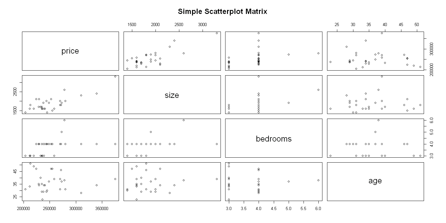
10.2. 10.2 TWO-WAY SCATTERPLOTS#

10.2.1. Figure 10.1#

pairs(~price+size+bedrooms+age,
   main="Simple Scatterplot Matrix")

_images/dc19acedddd882fb74a97d8c43ffc067f8e1f61385abe9ebd1995ad59a37dda4.png

10.3. 10.3 CORRELATION#

10.3.1. Table 10.3#

cor(cbind(price, size, bedrooms, bathrooms, lotsize, age, monthsold))

A matrix: 7 × 7 of type dbl
	price	size	bedrooms	bathrooms	lotsize	age	monthsold
price	1.00000000	0.78578205	0.42727531	0.32979279	0.15347859	-0.06801485	-0.20998489
size	0.78578205	1.00000000	0.51763025	0.31633817	0.11243727	0.07692458	-0.21451134
bedrooms	0.42727531	0.51763025	1.00000000	0.03743530	0.29220646	-0.02613989	0.18251169
bathrooms	0.32979279	0.31633817	0.03743530	1.00000000	0.10157490	0.03701787	-0.39230986
lotsize	0.15347859	0.11243727	0.29220646	0.10157490	1.00000000	-0.01922042	-0.05714046
age	-0.06801485	0.07692458	-0.02613989	0.03701787	-0.01922042	1.00000000	-0.36620679
monthsold	-0.20998489	-0.21451134	0.18251169	-0.39230986	-0.05714046	-0.36620679	1.00000000

10.4. 10.4 REGRESSION LINE#

Multivariate regression

ols.full = lm(price ~ size+bedrooms+bathrooms+lotsize+age+monthsold)
summ(ols.full, digits=3, confint='TRUE')

MODEL INFO:
Observations: 29
Dependent Variable: price
Type: OLS linear regression 

MODEL FIT:
F(6,22) = 6.826, p = 0.000
R² = 0.651
Adj. R² = 0.555 

Standard errors:OLS
-------------------------------------------------------------------------
                          Est.         2.5%        97.5%   t val.       p
----------------- ------------ ------------ ------------ -------- -------
(Intercept)         137791.066    10320.557   265261.574    2.242   0.035
size                    68.369       36.454      100.285    4.443   0.000
bedrooms              2685.315   -16378.816    21749.447    0.292   0.773
bathrooms             6832.880   -25770.876    39436.636    0.435   0.668
lotsize               2303.221   -12683.695    17290.138    0.319   0.753
age                   -833.039    -2324.847      658.770   -1.158   0.259
monthsold            -2088.504    -9390.399     5213.392   -0.593   0.559
-------------------------------------------------------------------------

Demonstrate that can get from bivariate regression on a residual

ols.size = lm(size ~ bedrooms+bathrooms+lotsize+age+monthsold)
resid.size = resid(ols.size)
summ(ols.biv <- lm(price ~ resid.size))

MODEL INFO:
Observations: 29
Dependent Variable: price
Type: OLS linear regression 

MODEL FIT:
F(1,27) = 12.33, p = 0.00
R² = 0.31
Adj. R² = 0.29 

Standard errors:OLS
-------------------------------------------------------
                         Est.      S.E.   t val.      p
----------------- ----------- --------- -------- ------
(Intercept)         253910.34   5858.45    43.34   0.00
resid.size              68.37     19.47     3.51   0.00
-------------------------------------------------------

10.5. 10.6 MODEL FIT#

Summary after lm saves a number of quantitites

sigma is the root mean squared error \((RMSE) = ResSS/(n-k)\)

R.squared is \(R^2\), adj.r.squared is adjusted \(R^2\), fstatistic is F statisic

df saves three things: \((k, N-k, k*)\) where k is effective number of parameters and \(k*>=k\) is the number of regressors including possibly nonidentified regressors if there is perfect collinearity

so k = df[1] and df = N-k = df[2]

R-squared is squared correlation between yhat and y

sum.full = summary(ols.full)
sum.full$r.squared
pprice = predict(ols.full)
print(describe(cbind(price,pprice)))
cor = cor(cbind(price,pprice))[2,1]
cor^2

0.650552844601402

       vars  n     mean       sd   median  trimmed      mad      min    max    range skew kurtosis      se
price     1 29 253910.3 37390.71 244000.0 249296.0 22239.00 204000.0 375000 171000.0 1.48     2.23 6943.28
pprice    2 29 253910.3 30158.17 251027.1 250698.4 21767.44 217089.5 357086 139996.6 1.42     2.55 5600.23

0.650552844601402

Compute Adjusted R-squared

k = sum.full$df[1]
df = sum.full$df[2]
r2 = sum.full$r.squared
r2adj = r2 - ((k-1)/df)*(1-r2)
r2adj
sum.full$adj.r.squared

0.555249074947239

Compute AIC and BIC manually

N = df + k
resSS = df*sum.full$sigma^2
# AIC as computed by many packages including Stata
aic = N*log(resSS/N) + N*(1+log(2*3.1415927)) + 2*k
aic

675.48240150411

AIC as computed by R drops the second term

aic_R = N*log(resSS/N) + 2*k
aic_R
extractAIC(ols.full)   # From summary(lm) output

593.183966149827

7
593.183966149827

BIC as computed by many packages including Stata

bic = N*log(resSS/N) + N*(1+log(2*3.1415927)) + k*log(N)
bic

685.053472314016

10.6. 10.7 COMPUTER OUTPUT FOLLOWING REGRESSION#

The following combines output from two models in a single table. It uses packages jtools which also needs huxtable for tables

library(huxtable)
# The two models
summ(ols.full <- lm(price ~ size+bedrooms+bathrooms+lotsize+age+monthsold))
summ(ols.small <- lm(price ~ size))

MODEL INFO:
Observations: 29
Dependent Variable: price
Type: OLS linear regression 

MODEL FIT:
F(6,22) = 6.83, p = 0.00
R² = 0.65
Adj. R² = 0.56 

Standard errors:OLS
--------------------------------------------------------
                         Est.       S.E.   t val.      p
----------------- ----------- ---------- -------- ------
(Intercept)         137791.07   61464.95     2.24   0.04
size                    68.37      15.39     4.44   0.00
bedrooms              2685.32    9192.53     0.29   0.77
bathrooms             6832.88   15721.19     0.43   0.67
lotsize               2303.22    7226.54     0.32   0.75
age                   -833.04     719.33    -1.16   0.26
monthsold            -2088.50    3520.90    -0.59   0.56
--------------------------------------------------------

MODEL INFO:
Observations: 29
Dependent Variable: price
Type: OLS linear regression 

MODEL FIT:
F(1,27) = 43.58, p = 0.00
R² = 0.62
Adj. R² = 0.60 

Standard errors:OLS
--------------------------------------------------------
                         Est.       S.E.   t val.      p
----------------- ----------- ---------- -------- ------
(Intercept)         115017.28   21489.36     5.35   0.00
size                    73.77      11.17     6.60   0.00
--------------------------------------------------------

Default includes standard errors

export_summs(ols.full, ols.onereg, scale = TRUE)

A huxtable: 18 × 3
	names	Model 1	Model 2
	<chr>	<chr>	<chr>
		Model 1	Model 2
1	(Intercept)	253910.344827586 ***	253910.344827586 ***
2		(4630.44948878858)	(6392.76419244658)
3	size	27229.6341330319 ***
4		(6129.19772656264)
5	bedrooms	1812.66731922359	15976.1273453258 *
6		(6205.2273627909)	(6505.91924598171)
7	bathrooms	2330.99683705654
8		(5363.19204846579)
9	lotsize	1596.20979166114
10		(5008.2316865653)
11	age	-5930.38085788559
12		(5120.92452909128)
13	monthsold	-3507.31651374698
14		(5912.79950609896)
1.1	N	29	29
2.1	R2	0.650552844601402	0.182564186920865
.1	All continuous predictors are mean-centered and scaled by 1 standard deviation. The outcome variable is in its original units. * p < 0.001; p < 0.01; * p < 0.05.	All continuous predictors are mean-centered and scaled by 1 standard deviation. The outcome variable is in its original units. * p < 0.001; p < 0.01; * p < 0.05.	All continuous predictors are mean-centered and scaled by 1 standard deviation. The outcome variable is in its original units. * p < 0.001; p < 0.01; * p < 0.05.

This gives t-statistics

export_summs(ols.full, ols.onereg, scale = TRUE, 
             error_format = "({statistic})")

A huxtable: 18 × 3
	names	Model 1	Model 2
	<chr>	<chr>	<chr>
		Model 1	Model 2
1	(Intercept)	253910.344827586 ***	253910.344827586 ***
2		(54.8349237892268)	(39.718396797366)
3	size	27229.6341330319 ***
4		(4.4426098402772)
5	bedrooms	1812.66731922359	15976.1273453258 *
6		(0.29211940405167)	(2.45562951848707)
7	bathrooms	2330.99683705654
8		(0.434628634587746)
9	lotsize	1596.20979166114
10		(0.318717242244006)
11	age	-5930.38085788559
12		(-1.15806839647722)
13	monthsold	-3507.31651374698
14		(-0.59317359063659)
1.1	N	29	29
2.1	R2	0.650552844601402	0.182564186920865
.1	All continuous predictors are mean-centered and scaled by 1 standard deviation. The outcome variable is in its original units. * p < 0.001; p < 0.01; * p < 0.05.	All continuous predictors are mean-centered and scaled by 1 standard deviation. The outcome variable is in its original units. * p < 0.001; p < 0.01; * p < 0.05.	All continuous predictors are mean-centered and scaled by 1 standard deviation. The outcome variable is in its original units. * p < 0.001; p < 0.01; * p < 0.05.

This gives t-statistics and p-values

export_summs(ols.full, ols.onereg, scale = TRUE, 
    error_format = "({statistic}, p = {p.value})")

A huxtable: 18 × 3
	names	Model 1	Model 2
	<chr>	<chr>	<chr>
		Model 1	Model 2
1	(Intercept)	253910.344827586 ***	253910.344827586 ***
2		(54.8349237892268, p = 0)	(39.718396797366, p = 0)
3	size	27229.6341330319 ***
4		(4.4426098402772, p = 0.000204637210605776)
5	bedrooms	1812.66731922359	15976.1273453258 *
6		(0.29211940405167, p = 0.772932358924004)	(2.45562951848707, p = 0.0207866997782178)
7	bathrooms	2330.99683705654
8		(0.434628634587746, p = 0.668065373738364)
9	lotsize	1596.20979166114
10		(0.318717242244006, p = 0.752947112842582)
11	age	-5930.38085788559
12		(-1.15806839647722, p = 0.259254037652819)
13	monthsold	-3507.31651374698
14		(-0.59317359063659, p = 0.55911430746301)
1.1	N	29	29
2.1	R2	0.650552844601402	0.182564186920865
.1	All continuous predictors are mean-centered and scaled by 1 standard deviation. The outcome variable is in its original units. * p < 0.001; p < 0.01; * p < 0.05.	All continuous predictors are mean-centered and scaled by 1 standard deviation. The outcome variable is in its original units. * p < 0.001; p < 0.01; * p < 0.05.	All continuous predictors are mean-centered and scaled by 1 standard deviation. The outcome variable is in its original units. * p < 0.001; p < 0.01; * p < 0.05.

This gives 95% confidence interval

export_summs(ols.full, ols.onereg, scale = TRUE,
             error_format = "[{conf.low}, {conf.high}]")

A huxtable: 18 × 3
	names	Model 1	Model 2
	<chr>	<chr>	<chr>
		Model 1	Model 2
1	(Intercept)	253910.344827586 ***	253910.344827586 ***
2		[244307.380340498, 263513.309314675]	[240793.476172862, 267027.21348231]
3	size	27229.6341330319 ***
4		[14518.456040055, 39940.8122260087]
5	bedrooms	1812.66731922359	15976.1273453258 *
6		[-11056.1865886896, 14681.5212271367]	[2627.08369866414, 29325.1709919875]
7	bathrooms	2330.99683705654
8		[-8791.58271025368, 13453.5763843668]
9	lotsize	1596.20979166114
10		[-8790.2270209302, 11982.6466042525]
11	age	-5930.38085788559
12		[-16550.5283215371, 4689.76660576591]
13	monthsold	-3507.31651374698
14		[-15769.7121653618, 8755.07913786788]
1.1	N	29	29
2.1	R2	0.650552844601402	0.182564186920865
.1	All continuous predictors are mean-centered and scaled by 1 standard deviation. The outcome variable is in its original units. * p < 0.001; p < 0.01; * p < 0.05.	All continuous predictors are mean-centered and scaled by 1 standard deviation. The outcome variable is in its original units. * p < 0.001; p < 0.01; * p < 0.05.	All continuous predictors are mean-centered and scaled by 1 standard deviation. The outcome variable is in its original units. * p < 0.001; p < 0.01; * p < 0.05.