2. CHAPTER 2. UNIVARIATE DATA SUMMARY#
Set up
library(foreign) # to open stata.dta files
library(psych) # for better sammary of descriptive statistics
library(repr) # to combine graphs with adjustable plot dimensions
options(repr.plot.width = 12, repr.plot.height = 6) # Plot dimensions (in inches)
options(width = 150) # To increase character width of printed output
2.1. 2.1 SUMMARY STATISTICS FOR NUMERICAL DATA#
rm(list=ls())
df = read.dta(file = "Dataset/AED_EARNINGS.DTA")
print(describe(df))
          vars   n     mean       sd median  trimmed      mad  min    max  range  skew kurtosis      se
earnings     1 171 41412.69 25527.05  36000 38052.70 17049.90 1050 172000 170950  1.70     4.23 1952.10
education    2 171    14.43     2.74     14    14.45     2.97    3     20     17 -0.45     1.16    0.21
age          3 171    30.00     0.00     30    30.00     0.00   30     30      0   NaN      NaN    0.00
gender       4 171     0.00     0.00      0     0.00     0.00    0      0      0   NaN      NaN    0.00
2.1.1. Table 2.1#
print(describe(df$earnings))
   vars   n     mean       sd median trimmed     mad  min    max  range skew kurtosis     se
X1    1 171 41412.69 25527.05  36000 38052.7 17049.9 1050 172000 170950  1.7     4.23 1952.1
quantile(df$earnings)
- 0%
- 1050
- 25%
- 25000
- 50%
- 36000
- 75%
- 49000
- 100%
- 172000
mean(df$earnings)
41412.6900584795
Skewness and kurtosis require moments package
attach(df) # Allow variables in database to be accessed simply by giving names
library(moments)

skewness(earnings) #Note no need to write "df$..." now since we've attached the data.
kurtosis(earnings)
1.71255481120525
7.3163879423401
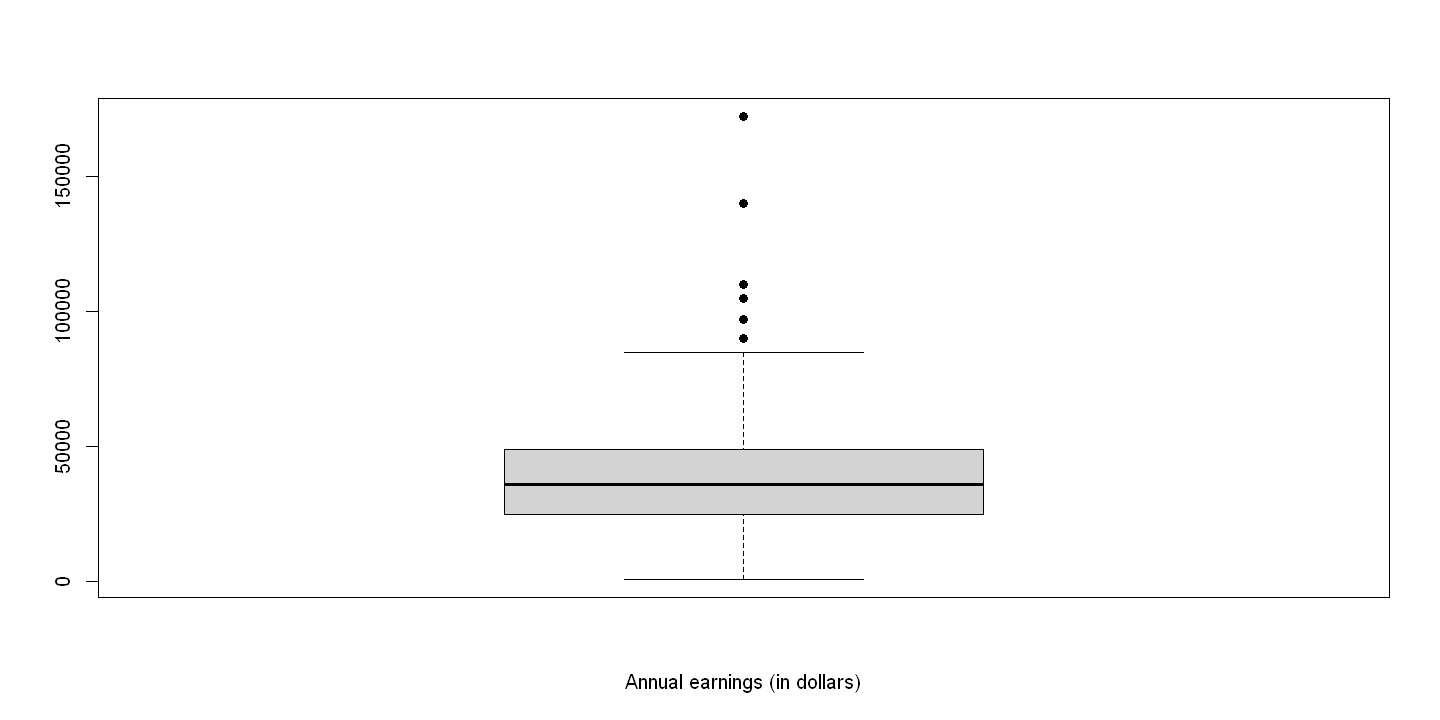
2.1.2. Figure 2.2#
boxplot(earnings,xlab="Annual earnings (in dollars)",pch=19)
2.2. 2.2 CHARTS FOR NUMERICAL DATA#
2.2.1. Table 2.2#
print(describe(earnings))
   vars   n     mean       sd median trimmed     mad  min    max  range skew kurtosis     se
X1    1 171 41412.69 25527.05  36000 38052.7 17049.9 1050 172000 170950  1.7     4.23 1952.1
# Define bins
bins <- cut(earnings, breaks = seq(0, 180000, by = 15000), right = FALSE)

# Frequency table
freq <- table(bins)

# Relative frequency (%)
rel_freq <- prop.table(freq) * 100

# Combine
result <- data.frame(
  Range = names(freq),
  Frequency = as.numeric(freq),
  `Relative Frequency (%)` = round(as.numeric(rel_freq), 2)
)

print(result)
                Range Frequency Relative.Frequency....
1         [0,1.5e+04)        12                   7.02
2     [1.5e+04,3e+04)        53                  30.99
3     [3e+04,4.5e+04)        52                  30.41
4     [4.5e+04,6e+04)        20                  11.70
5     [6e+04,7.5e+04)        11                   6.43
6     [7.5e+04,9e+04)        16                   9.36
7    [9e+04,1.05e+05)         2                   1.17
8  [1.05e+05,1.2e+05)         3                   1.75
9  [1.2e+05,1.35e+05)         0                   0.00
10 [1.35e+05,1.5e+05)         1                   0.58
11 [1.5e+05,1.65e+05)         0                   0.00
12 [1.65e+05,1.8e+05)         1                   0.58
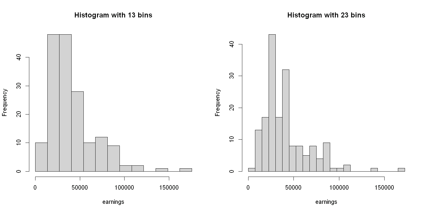
2.2.2. Figure 2.4#
par(mfrow = c(1, 2)) # Sets layout to 1 row, 2 columns

hist(earnings,breaks=c(13500*0:13), main = "Histogram with 13 bins") # 13 bins

hist(earnings,breaks=c(7500*0:23), main = "Histogram with 23 bins") # 23 bins
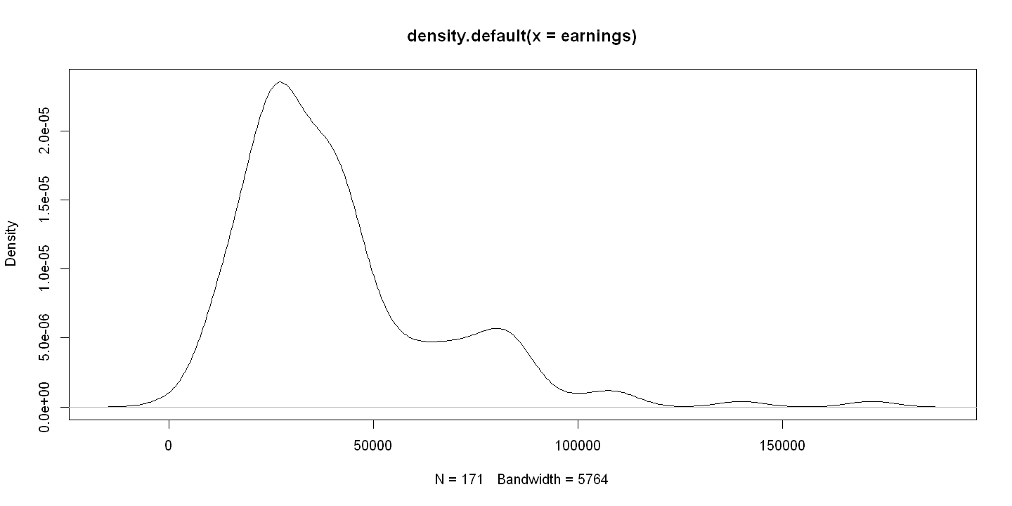
2.2.3. Figure 2.5#
# Default kernel density estiamte in R
kdensity = density(earnings)
plot(kdensity)
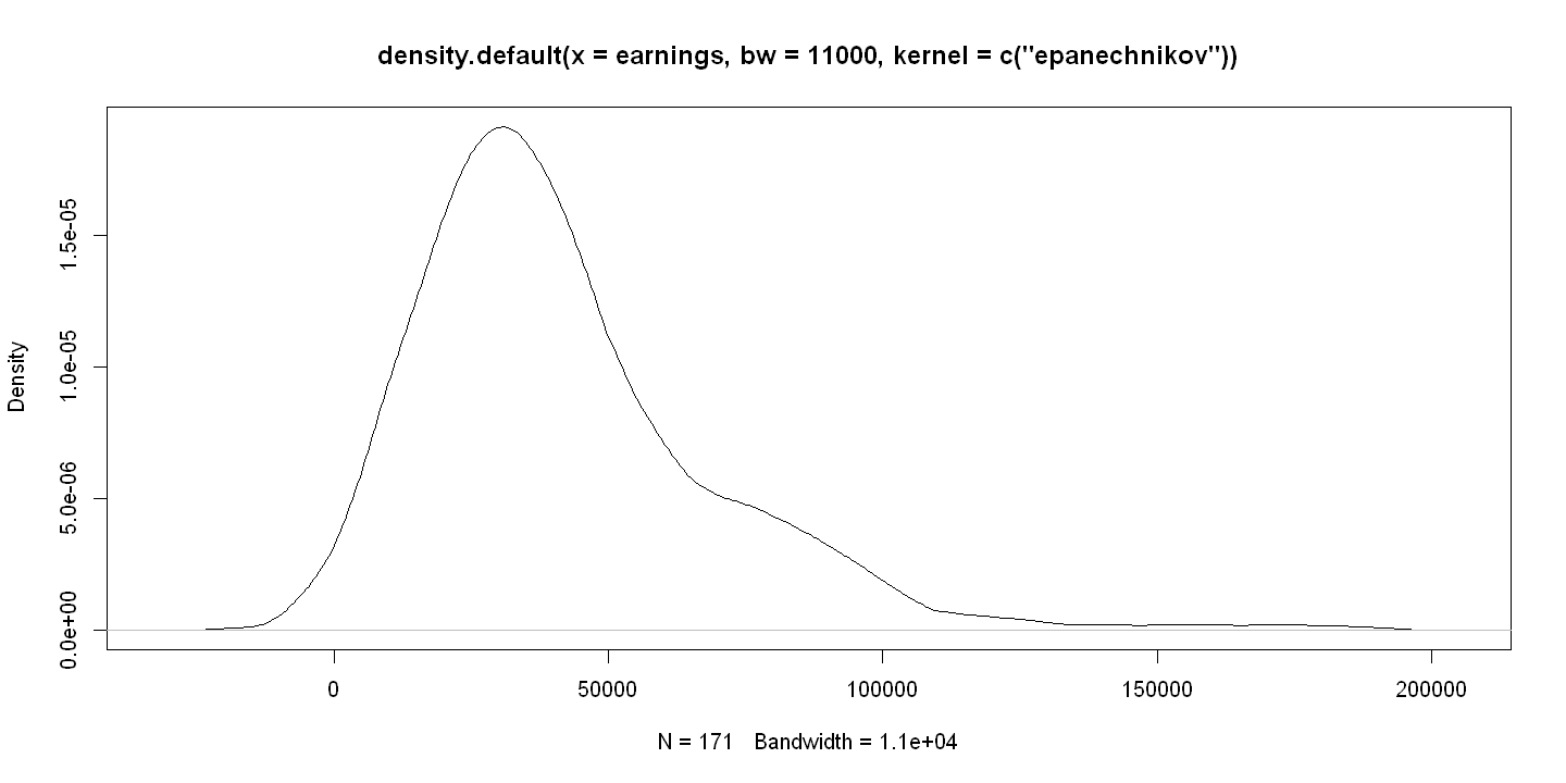
# Select kernel and band width
kdensity = density(earnings,kernel=c("epanechnikov"),bw=11000)
plot( kdensity)
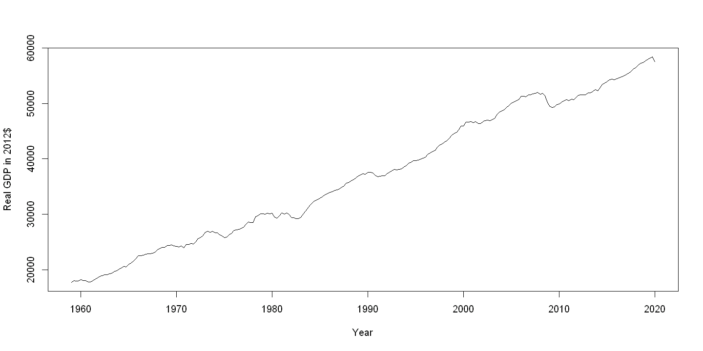
2.2.4. Figure 2.6#
(New dataset)
rm(list=ls())
df = read.dta(file = "Dataset/AED_REALGDPPC.DTA")
#df<-na.omit(df)
print(describe(df))
Warning message in FUN(newX[, i], ...):
"no non-missing arguments to min; returning Inf"
Warning message in FUN(newX[, i], ...):
"no non-missing arguments to max; returning -Inf"
          vars   n      mean       sd    median   trimmed      mad       min       max     range  skew kurtosis      se
gdpc1        1 245   9925.24  4814.02   9238.92   9716.91  6140.55   3121.94  19221.97  16100.03  0.32    -1.25  307.56
gdp          2 245   7401.46  6331.00   5695.36   6755.00  6885.44    510.33  21729.12  21218.79  0.65    -0.88  404.47
gdpdef       3 245     59.72    31.20     61.65     59.06    44.57     16.35    113.50     97.16  0.03    -1.36    1.99
date*        4 245    123.00    70.87    123.00    123.00    90.44      1.00    245.00    244.00  0.00    -1.21    4.53
daten        5 245       NaN       NA        NA       NaN       NA       Inf      -Inf      -Inf    NA       NA      NA
quarter      6 245    118.00    70.87    118.00    118.00    90.44     -4.00    240.00    244.00  0.00    -1.21    4.53
popthm       7 245 253116.88 45611.79 247695.00 252742.75 58854.77 176044.00 329527.00 153483.00  0.10    -1.28 2914.03
year         8 245   1989.13    17.72   1989.00   1989.13    22.24   1959.00   2020.00     61.00  0.00    -1.21    1.13
realgdp      9 245   9925.24  4814.03   9238.97   9716.90  6140.78   3121.86  19222.00  16100.14  0.32    -1.25  307.56
gdppc       10 245  25841.47 19184.69  22993.15  24423.21 24740.38   2898.86  66008.59  63109.73  0.44    -1.13 1225.66
realgdppc   11 245  37050.50 12089.68  36929.01  36996.63 16507.15  17733.26  58392.45  40659.20  0.08    -1.33  772.38
growth      12 241      1.99     2.18      2.09      2.08     1.80     -4.77      7.63     12.40 -0.38     0.64    0.14
plot(df$daten, df$realgdppc, xlab="Year", ylab="Real GDP in 2012$", type="l")
2.3. 2.3 CHARTS FOR NUMERICAL DATA BY CATEGORY#
2.3.1. Figure 2.7#
Uses new data
rm(list=ls())
df = read.dta(file = "Dataset/AED_HEALTHCATEGORIES.DTA")
print(describe(df))
vars n mean sd median trimmed mad min max range skew kurtosis se
category* 1 13 7.0 3.89 7 7.00 4.45 1 13 12 0.00 -1.48 1.08
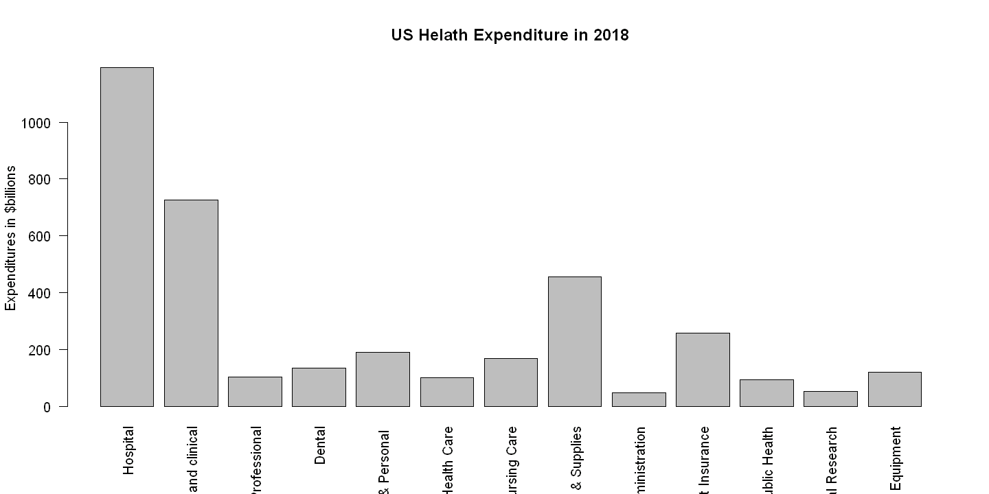
expenditures 2 13 281.0 332.97 136 219.36 83.03 48 1192 1144 1.66 1.63 92.35
cat_short* 3 13 3.0 2.00 3 2.82 2.97 1 7 6 0.63 -0.98 0.55
exp_short 4 4 539.5 520.58 431 539.50 461.09 104 1192 1088 0.24 -2.17 260.29
2.3.2. Table 2.3#
attach(df)
df[, c("category","expenditures")]
| category | expenditures | |
|---|---|---|
| <chr> | <int> | |
| 1 | Hospital | 1192 |
| 2 | Physician and clinical | 726 |
| 3 | Other Professional | 104 |
| 4 | Dental | 136 |
| 5 | Other Health & Personal | 192 |
| 6 | Home Health Care | 102 |
| 7 | Nursing Care | 169 |
| 8 | Drugs & Supplies | 456 |
| 9 | Govt. Administration | 48 |
| 10 | Net Cost Insurance | 259 |
| 11 | Govt. Public Health | 94 |
| 12 | Noncommercial Research | 53 |
| 13 | Structures & Equipment | 122 |
2.3.3. Figure 2.7#
barplot(expenditures,names.arg=category,las=2,ylab="Expenditures in $billions", main="US Helath Expenditure in 2018")
2.4. 2.4 SUMMARY AND CHARTS FOR CATEGORICAL DATA#
2.4.1. Table 2.4#
rm(list=ls())
df = read.dta(file = "Dataset/AED_FISHING.DTA")
attach(df)
print(describe(df))
         vars    n   mean     sd median trimmed   mad   min    max  range  skew kurtosis   se
mode*       1 1182   3.01   0.99   3.00    3.13  1.48  1.00   4.00   3.00 -0.70    -0.58 0.03
price       2 1182  52.08  53.83  37.90   42.52 35.13  1.29 666.11 664.82  3.14    19.19 1.57
crate       3 1182   0.39   0.56   0.16    0.26  0.23  0.00   2.31   2.31  2.35     5.23 0.02
dbeach      4 1182   0.11   0.32   0.00    0.02  0.00  0.00   1.00   1.00  2.44     3.94 0.01
dpier       5 1182   0.15   0.36   0.00    0.06  0.00  0.00   1.00   1.00  1.95     1.81 0.01
dprivate    6 1182   0.35   0.48   0.00    0.32  0.00  0.00   1.00   1.00  0.61    -1.63 0.01
dcharter    7 1182   0.38   0.49   0.00    0.35  0.00  0.00   1.00   1.00  0.48    -1.77 0.01
pbeach      8 1182 103.42 103.64  74.63   85.99 78.33  1.29 843.19 841.90  1.87     4.97 3.01
ppier       9 1182 103.42 103.64  74.63   85.99 78.33  1.29 843.19 841.90  1.87     4.97 3.01
pprivate   10 1182  55.26  62.71  33.53   43.05 34.45  2.29 666.11 663.82  2.65    12.26 1.82
pcharter   11 1182  84.38  63.54  61.61   72.35 35.45 27.29 691.11 663.82  2.59    11.64 1.85
qbeach     12 1182   0.24   0.19   0.25    0.23  0.28  0.07   0.53   0.47  0.63    -1.24 0.01
qpier      13 1182   0.16   0.16   0.08    0.15  0.11  0.00   0.45   0.45  1.07    -0.47 0.00
qprivate   14 1182   0.17   0.21   0.09    0.13  0.11  0.00   0.74   0.74  1.67     1.73 0.01
qcharter   15 1182   0.63   0.71   0.42    0.50  0.59  0.00   2.31   2.31  1.36     0.91 0.02
income     16 1182   4.10   2.46   3.75    3.81  2.47  0.42  12.50  12.08  1.30     2.09 0.07
one        17 1182   1.00   0.00   1.00    1.00  0.00  1.00   1.00   0.00   NaN      NaN 0.00
freq = table(mode)
relfreq = table(mode) / nrow(df)
relfreq
cbind(freq,relfreq)
mode
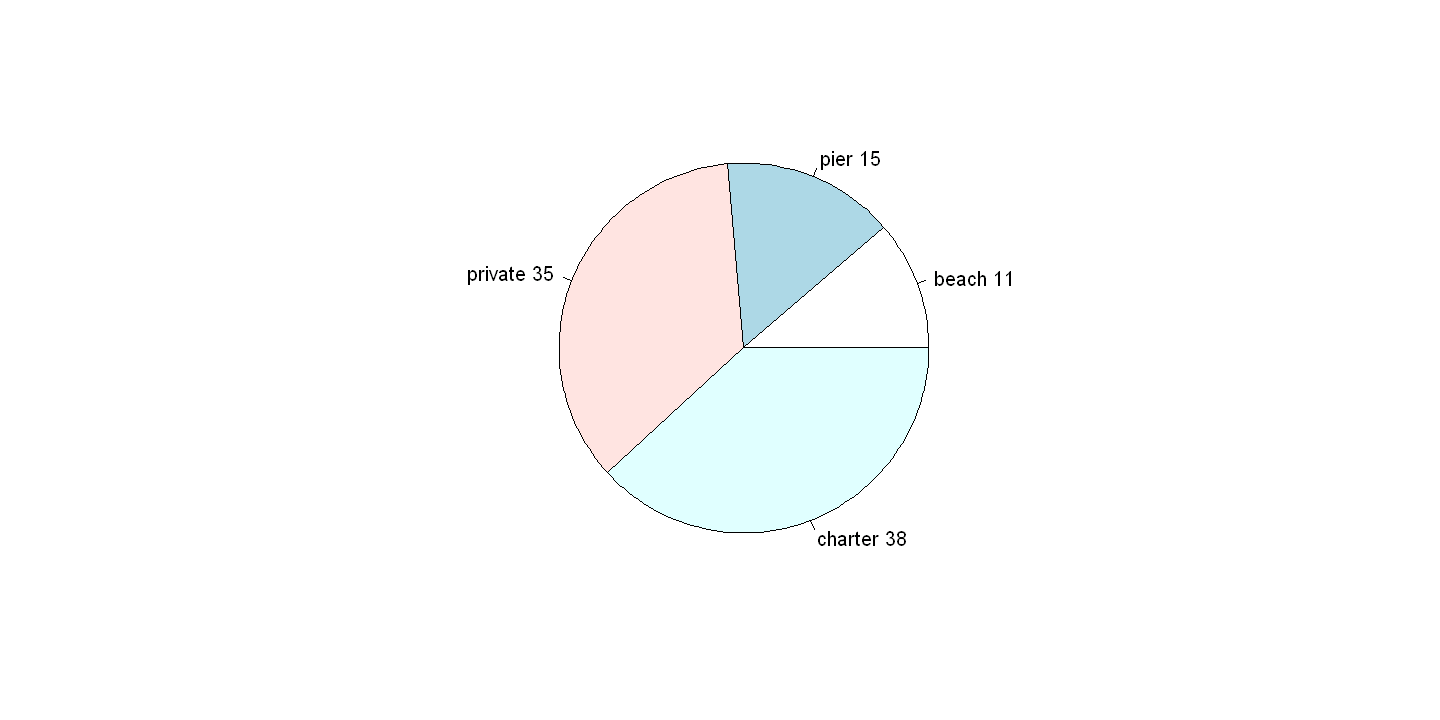
beach pier private charter
0.1133672 0.1505922 0.3536379 0.3824027
| freq | relfreq | |
|---|---|---|
| beach | 134 | 0.1133672 |
| pier | 178 | 0.1505922 |
| private | 418 | 0.3536379 |
| charter | 452 | 0.3824027 |
2.4.2. Figure 2.9#
lbls = c("beach","pier","private","charter")
pct <- round(freq/sum(freq)*100)
lbls <- paste(lbls, pct) # add percents to labels
pie(freq,labels=lbls)
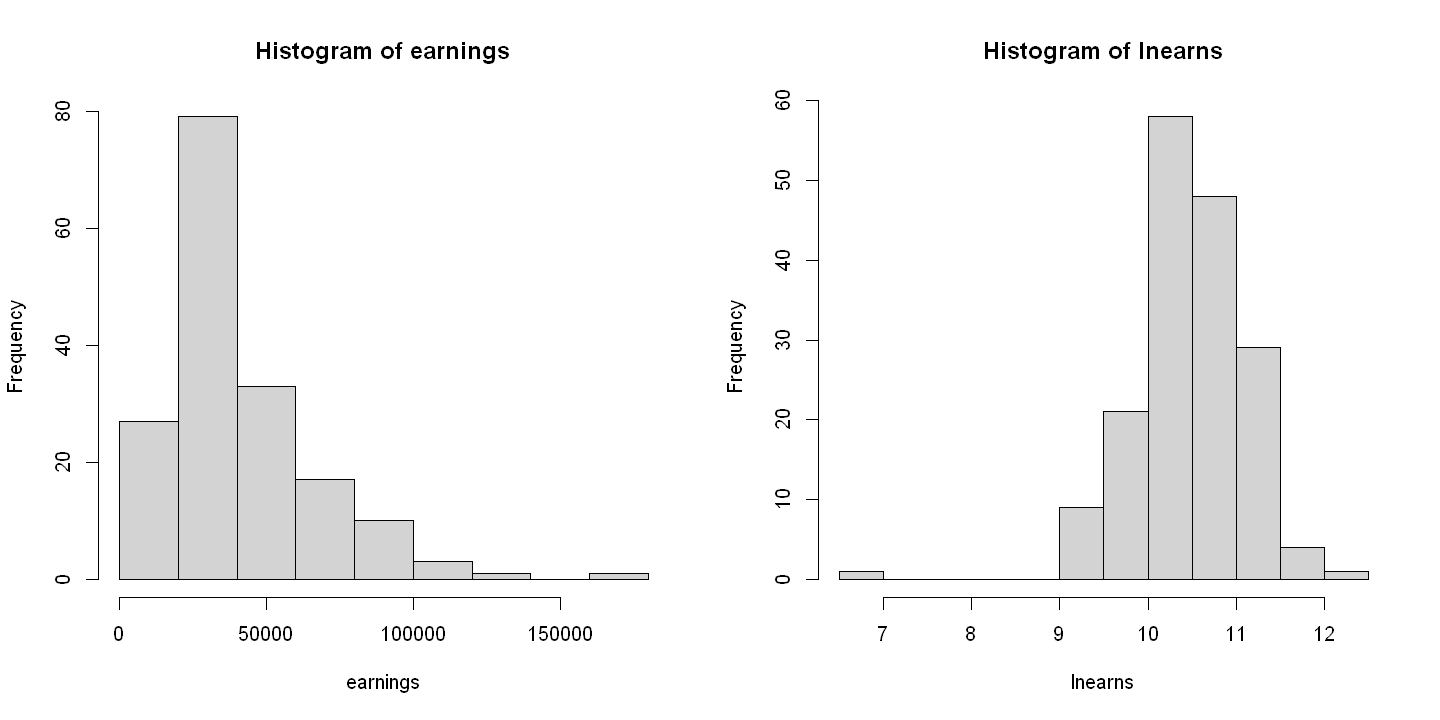
2.5. 2.5 DATA TRANSFORMATION#
2.5.1. Figure 2.10#
rm(list=ls())
df = read.dta(file = "Dataset/AED_EARNINGS.DTA")
print(describe(df))

lnearns = log(earnings)

# Following combines into one graph
par(mfrow=c(1,2))
hist(earnings)
hist(lnearns)
par(mfrow=c(1,1))
          vars   n     mean       sd median  trimmed      mad  min    max  range  skew kurtosis      se
earnings     1 171 41412.69 25527.05  36000 38052.70 17049.90 1050 172000 170950  1.70     4.23 1952.10
education    2 171    14.43     2.74     14    14.45     2.97    3     20     17 -0.45     1.16    0.21
age          3 171    30.00     0.00     30    30.00     0.00   30     30      0   NaN      NaN    0.00
gender       4 171     0.00     0.00      0     0.00     0.00    0      0      0   NaN      NaN    0.00
2.6. 2.6 DATA TRANSFORMATIONS FOR TIME SERIES DATA#
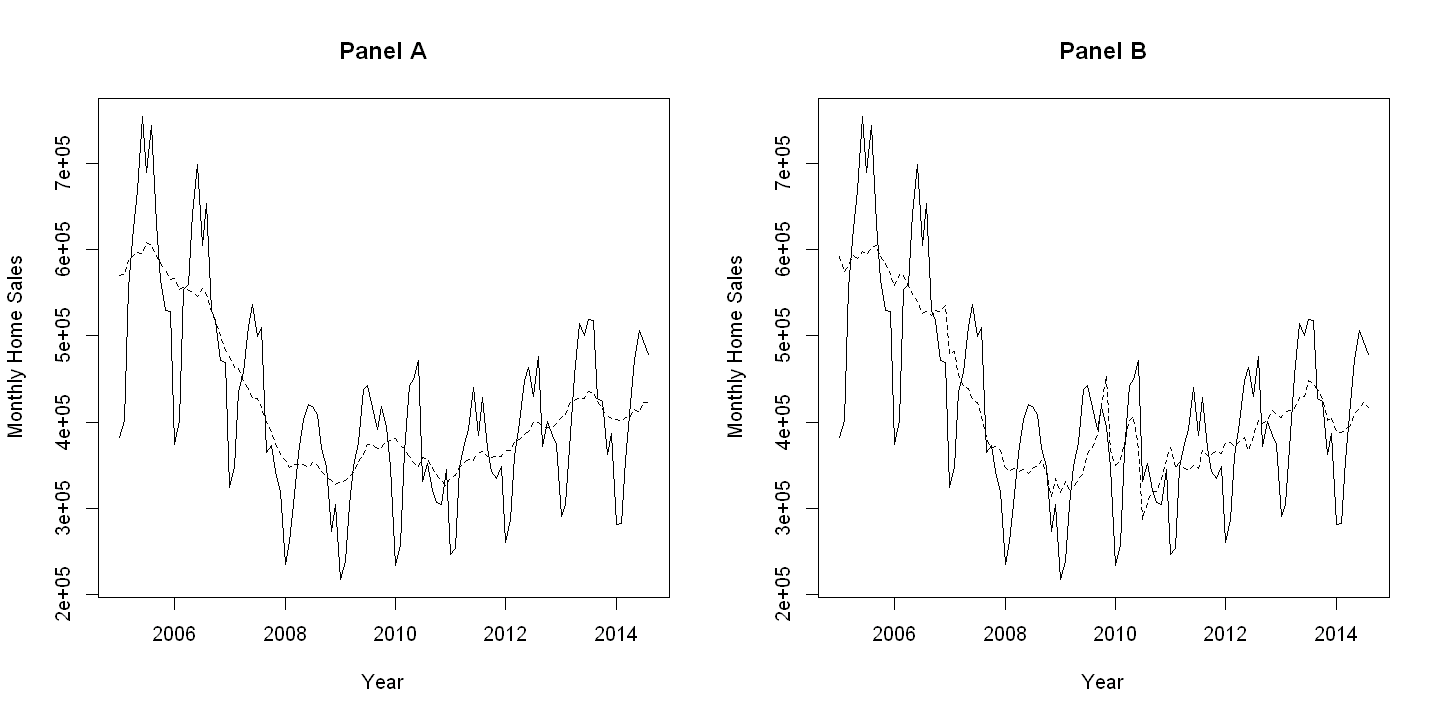
2.6.1. Figure 2.11#
rm(list=ls())
df = read.dta(file = "Dataset/AED_MONTHLYHOMESALES.DTA")
df<-na.omit(df)
print(describe(df))
Warning message in FUN(newX[, i], ...):
"no non-missing arguments to min; returning Inf"
Warning message in FUN(newX[, i], ...):
"no non-missing arguments to max; returning -Inf"
             vars   n      mean        sd    median   trimmed       mad       min      max     range skew kurtosis      se
date*           1 183     92.00     52.97     92.00     92.00     68.20      1.00    183.0    182.00 0.00    -1.22    3.92
daten           2 183       NaN        NA        NA       NaN        NA       Inf     -Inf      -Inf   NA       NA      NA
year            3 183   2006.54      4.43   2007.00   2006.54      5.93   1999.00   2014.0     15.00 0.00    -1.20    0.33
month           4 183    564.00     52.97    564.00    564.00     68.20    473.00    655.0    182.00 0.00    -1.22    3.92
exsales         5 183 441896.17 112222.28 430000.00 436442.18 120090.60 218000.00 754000.0 536000.00 0.42    -0.20 8295.71
exsales_sa      6 183 440405.28  79738.96 429166.66 436553.29  87720.53 287500.00 605000.0 317500.00 0.40    -0.85 5894.47
exsales_ma11    7 183 440587.18  77367.04 429818.19 435697.59  83025.60 324818.19 608545.4 283727.25 0.50    -0.84 5719.14
construct       8 183  77758.60  13800.18  76605.00  77087.00  13432.36  50590.00 110434.0  59844.00 0.40    -0.44 1020.14
construct_sa    9 183  77654.14  10938.52  73654.41  76862.75   9539.67  61597.25 101105.8  39508.59 0.61    -0.94  808.60
newdata <- df[which(df$year>=2005),]
attach(newdata)
print(describe(newdata))
Warning message in FUN(newX[, i], ...):
"no non-missing arguments to min; returning Inf"
Warning message in FUN(newX[, i], ...):
"no non-missing arguments to max; returning -Inf"
             vars   n      mean        sd    median   trimmed      mad       min      max     range skew kurtosis       se
date*           1 116     58.50     33.63     58.50     58.50    43.00      1.00    116.0    115.00 0.00    -1.23     3.12
daten           2 116       NaN        NA        NA       NaN       NA       Inf     -Inf      -Inf   NA       NA       NA
year            3 116   2009.34      2.81   2009.00   2009.34     2.97   2005.00   2014.0      9.00 0.02    -1.23     0.26
month           4 116    597.50     33.63    597.50    597.50    43.00    540.00    655.0    115.00 0.00    -1.23     3.12
exsales         5 116 418224.14 113429.85 400500.00 409329.79 99334.20 218000.00 754000.0 536000.00 0.75     0.39 10531.70
exsales_sa      6 116 418060.34  85092.86 393750.00 409326.24 66099.27 287500.00 605000.0 317500.00 0.91    -0.40  7900.67
exsales_ma11    7 116 418300.16  81757.24 394000.00 408255.32 56743.13 324818.19 608545.4 283727.25 1.05    -0.23  7590.97
construct       8 116  80910.13  14761.47  80222.00  80769.12 14440.52  50590.00 110434.0  59844.00 0.14    -0.76  1370.57
construct_sa    9 116  81005.70  11693.50  79465.54  80859.19 16730.90  62914.17 101105.8  38191.67 0.16    -1.46  1085.71
par(mfrow=c(1,2))
plot(daten, exsales, main="Panel A", xlab="Year", ylab="Monthly Home Sales", type="l")
points(daten, exsales_ma11, type="l",lty=2)
plot(daten, exsales, main="Panel B", xlab="Year", ylab="Monthly Home Sales", type="l")
points(daten, exsales_sa, type="l",lty=2)
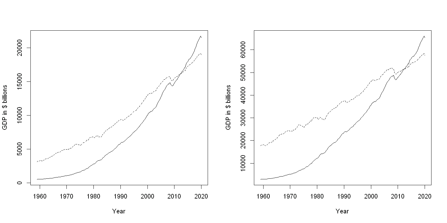
2.6.2. Figure 2.12#
rm(list=ls())
df = read.dta(file = "Dataset/AED_REALGDPPC.DTA")
attach(df)
print(describe(df))
The following objects are masked from newdata:

    date, daten, year
Warning message in FUN(newX[, i], ...):
"no non-missing arguments to min; returning Inf"
Warning message in FUN(newX[, i], ...):
"no non-missing arguments to max; returning -Inf"
          vars   n      mean       sd    median   trimmed      mad       min       max     range  skew kurtosis      se
gdpc1        1 245   9925.24  4814.02   9238.92   9716.91  6140.55   3121.94  19221.97  16100.03  0.32    -1.25  307.56
gdp          2 245   7401.46  6331.00   5695.36   6755.00  6885.44    510.33  21729.12  21218.79  0.65    -0.88  404.47
gdpdef       3 245     59.72    31.20     61.65     59.06    44.57     16.35    113.50     97.16  0.03    -1.36    1.99
date*        4 245    123.00    70.87    123.00    123.00    90.44      1.00    245.00    244.00  0.00    -1.21    4.53
daten        5 245       NaN       NA        NA       NaN       NA       Inf      -Inf      -Inf    NA       NA      NA
quarter      6 245    118.00    70.87    118.00    118.00    90.44     -4.00    240.00    244.00  0.00    -1.21    4.53
popthm       7 245 253116.88 45611.79 247695.00 252742.75 58854.77 176044.00 329527.00 153483.00  0.10    -1.28 2914.03
year         8 245   1989.13    17.72   1989.00   1989.13    22.24   1959.00   2020.00     61.00  0.00    -1.21    1.13
realgdp      9 245   9925.24  4814.03   9238.97   9716.90  6140.78   3121.86  19222.00  16100.14  0.32    -1.25  307.56
gdppc       10 245  25841.47 19184.69  22993.15  24423.21 24740.38   2898.86  66008.59  63109.73  0.44    -1.13 1225.66
realgdppc   11 245  37050.50 12089.68  36929.01  36996.63 16507.15  17733.26  58392.45  40659.20  0.08    -1.33  772.38
growth      12 241      1.99     2.18      2.09      2.08     1.80     -4.77      7.63     12.40 -0.38     0.64    0.14
2.6.3. #
par(mfrow=c(1,2))
plot(daten, gdp, xlab="Year", ylab="GDP in $ billions", type="l",lty=1)
points(daten, realgdp, type="l",lty=2)
plot(daten, gdppc, xlab="Year", ylab="GDP in $ billions", type="l",lty=1)
points(daten, realgdppc, type="l",lty=2)
par(mfrow=c(1,1))
2.6.4. Table 2.5#
selected_cols <- c("date", "quarter", "gdp", "gdpdef", "realgdp")

first_row <- head(df[, selected_cols], n = 1)
last_row  <- tail(df[, selected_cols], n = 1)

# Combine
result <- rbind(first_row, last_row)
print(result)
          date quarter      gdp  gdpdef   realgdp
1   1959-01-01      -4   510.33  16.347  3121.857
245 2020-01-01     240 21539.69 113.502 18977.365