9 CHAPTER 9: MODELLING VOLATILITY AND CORRELATION
9.1 Estimating the GARCH(1,1) model (Page 438)
library("foreign")
data = read.dta("Dataset/currencies.dta")
data = na.omit(data)

library("rugarch")
garch11.spec = ugarchspec(mean.model=list(armaOrder=c(0,0)),
                          variance.model=list(garchOrder=c(1,1),model="sGARCH"))
garch11.fit = ugarchfit(garch11.spec,data=data$rjpy)
garch11.fit
##
## *---------------------------------*
## *          GARCH Model Fit        *
## *---------------------------------*
##
## Conditional Variance Dynamics
## -----------------------------------
## GARCH Model  : sGARCH(1,1)
## Mean Model   : ARFIMA(0,0,0)
## Distribution : norm
##
## Optimal Parameters
## ------------------------------------
##         Estimate  Std. Error  t value Pr(>|t|)
## mu      0.002546    0.006769  0.37612 0.706828
## omega   0.004489    0.001126  3.98853 0.000066
## alpha1  0.047579    0.008082  5.88696 0.000000
## beta1   0.932508    0.011884 78.46766 0.000000
##
## Robust Standard Errors:
##         Estimate  Std. Error  t value Pr(>|t|)
## mu      0.002546    0.008090  0.31472 0.752974
## omega   0.004489    0.002849  1.57558 0.115123
## alpha1  0.047579    0.019477  2.44282 0.014573
## beta1   0.932508    0.028282 32.97212 0.000000
##
## LogLikelihood : -2460.987
##
## Information Criteria
## ------------------------------------
##
## Akaike       1.2365
## Bayes        1.2428
## Shibata      1.2365
## Hannan-Quinn 1.2387
##
## Weighted Ljung-Box Test on Standardized Residuals
## ------------------------------------
##                         statistic p-value
## Lag[1]                      102.5       0
## Lag[2*(p+q)+(p+q)-1][2]     103.6       0
## Lag[4*(p+q)+(p+q)-1][5]     106.8       0
## d.o.f=0
## H0 : No serial correlation
##
## Weighted Ljung-Box Test on Standardized Squared Residuals
## ------------------------------------
##                         statistic   p-value
## Lag[1]                      13.72 2.119e-04
## Lag[2*(p+q)+(p+q)-1][5]     17.81 7.692e-05
## Lag[4*(p+q)+(p+q)-1][9]     21.34 9.024e-05
## d.o.f=2
##
## Weighted ARCH LM Tests
## ------------------------------------
##             Statistic Shape Scale P-Value
## ARCH Lag[3]     3.514 0.500 2.000 0.06087
## ARCH Lag[5]     7.623 1.440 1.667 0.02472
## ARCH Lag[7]     9.455 2.315 1.543 0.02460
##
## Nyblom stability test
## ------------------------------------
## Joint Statistic:  0.7864
## Individual Statistics:
## mu     0.18508
## omega  0.08219
## alpha1 0.09814
## beta1  0.11643
##
## Asymptotic Critical Values (10% 5% 1%)
## Joint Statistic:          1.07 1.24 1.6
## Individual Statistic:     0.35 0.47 0.75
##
## Sign Bias Test
## ------------------------------------
##                     t-value      prob sig
## Sign Bias           0.08355 9.334e-01
## Negative Sign Bias  4.82315 1.466e-06 ***
## Positive Sign Bias  1.65357 9.829e-02   *
## Joint Effect       29.68720 1.606e-06 ***
##
##
## Adjusted Pearson Goodness-of-Fit Test:
## ------------------------------------
##   group statistic p-value(g-1)
## 1    20     847.9   1.378e-167
## 2    30    1084.9   9.530e-210
## 3    40    1291.6   1.213e-245
## 4    50    1426.0   2.061e-266
##
##
## Elapsed time : 0.2749989
9.2 GJR (‘threshold’ GARCH) (Page 442)
gjrgarch11.spec = ugarchspec(mean.model=list(armaOrder=c(0,0)),
                          variance.model=list(garchOrder=c(1,1),model="gjrGARCH"))
gjrgarch11.fit = ugarchfit(gjrgarch11.spec,data=data$rjpy)
gjrgarch11.fit
##
## *---------------------------------*
## *          GARCH Model Fit        *
## *---------------------------------*
##
## Conditional Variance Dynamics
## -----------------------------------
## GARCH Model  : gjrGARCH(1,1)
## Mean Model   : ARFIMA(0,0,0)
## Distribution : norm
##
## Optimal Parameters
## ------------------------------------
##         Estimate  Std. Error  t value Pr(>|t|)
## mu     -0.001369    0.006765 -0.20233 0.839658
## omega   0.003956    0.000938  4.21785 0.000025
## alpha1  0.025541    0.006127  4.16871 0.000031
## beta1   0.937628    0.010070 93.11060 0.000000
## gamma1  0.038786    0.008537  4.54342 0.000006
##
## Robust Standard Errors:
##         Estimate  Std. Error  t value Pr(>|t|)
## mu     -0.001369    0.008004 -0.17102 0.864209
## omega   0.003956    0.002096  1.88760 0.059080
## alpha1  0.025541    0.011676  2.18744 0.028710
## beta1   0.937628    0.020423 45.90967 0.000000
## gamma1  0.038786    0.017662  2.19596 0.028095
##
## LogLikelihood : -2447.737
##
## Information Criteria
## ------------------------------------
##
## Akaike       1.2304
## Bayes        1.2383
## Shibata      1.2304
## Hannan-Quinn 1.2332
##
## Weighted Ljung-Box Test on Standardized Residuals
## ------------------------------------
##                         statistic p-value
## Lag[1]                      108.4       0
## Lag[2*(p+q)+(p+q)-1][2]     109.3       0
## Lag[4*(p+q)+(p+q)-1][5]     112.7       0
## d.o.f=0
## H0 : No serial correlation
##
## Weighted Ljung-Box Test on Standardized Squared Residuals
## ------------------------------------
##                         statistic   p-value
## Lag[1]                      10.95 0.0009360
## Lag[2*(p+q)+(p+q)-1][5]     15.34 0.0003597
## Lag[4*(p+q)+(p+q)-1][9]     19.76 0.0002321
## d.o.f=2
##
## Weighted ARCH LM Tests
## ------------------------------------
##             Statistic Shape Scale P-Value
## ARCH Lag[3]     3.393 0.500 2.000 0.06547
## ARCH Lag[5]     8.179 1.440 1.667 0.01818
## ARCH Lag[7]    10.879 2.315 1.543 0.01146
##
## Nyblom stability test
## ------------------------------------
## Joint Statistic:  1.4159
## Individual Statistics:
## mu     0.14156
## omega  0.09306
## alpha1 0.10686
## beta1  0.11944
## gamma1 0.08167
##
## Asymptotic Critical Values (10% 5% 1%)
## Joint Statistic:          1.28 1.47 1.88
## Individual Statistic:     0.35 0.47 0.75
##
## Sign Bias Test
## ------------------------------------
##                    t-value      prob sig
## Sign Bias            1.393 1.638e-01
## Negative Sign Bias   3.204 1.364e-03 ***
## Positive Sign Bias   2.727 6.429e-03 ***
## Joint Effect        23.302 3.494e-05 ***
##
##
## Adjusted Pearson Goodness-of-Fit Test:
## ------------------------------------
##   group statistic p-value(g-1)
## 1    20     818.6   2.444e-161
## 2    30     998.8   1.574e-191
## 3    40    1138.9   1.757e-213
## 4    50    1275.1   8.706e-235
##
##
## Elapsed time : 0.4268448
9.3 EGARCH (Page 443)
egarch11.spec = ugarchspec(mean.model=list(armaOrder=c(0,0)),
                             variance.model=list(garchOrder=c(1,1),model="eGARCH"))
egarch11.fit = ugarchfit(egarch11.spec,data=data$rjpy)
egarch11.fit
##
## *---------------------------------*
## *          GARCH Model Fit        *
## *---------------------------------*
##
## Conditional Variance Dynamics
## -----------------------------------
## GARCH Model  : eGARCH(1,1)
## Mean Model   : ARFIMA(0,0,0)
## Distribution : norm
##
## Optimal Parameters
## ------------------------------------
##         Estimate  Std. Error   t value Pr(>|t|)
## mu     -0.001276    0.002104  -0.60618 0.544393
## omega  -0.022104    0.013013  -1.69861 0.089393
## alpha1 -0.037615    0.011148  -3.37416 0.000740
## beta1   0.979362    0.009578 102.24797 0.000000
## gamma1  0.108134    0.025814   4.18895 0.000028
##
## Robust Standard Errors:
##         Estimate  Std. Error  t value Pr(>|t|)
## mu     -0.001276    0.000962 -1.32584  0.18489
## omega  -0.022104    0.059750 -0.36994  0.71142
## alpha1 -0.037615    0.050061 -0.75138  0.45243
## beta1   0.979362    0.044902 21.81124  0.00000
## gamma1  0.108134    0.114671  0.94300  0.34568
##
## LogLikelihood : -2443.073
##
## Information Criteria
## ------------------------------------
##
## Akaike       1.2280
## Bayes        1.2359
## Shibata      1.2280
## Hannan-Quinn 1.2308
##
## Weighted Ljung-Box Test on Standardized Residuals
## ------------------------------------
##                         statistic p-value
## Lag[1]                      111.3       0
## Lag[2*(p+q)+(p+q)-1][2]     112.3       0
## Lag[4*(p+q)+(p+q)-1][5]     115.8       0
## d.o.f=0
## H0 : No serial correlation
##
## Weighted Ljung-Box Test on Standardized Squared Residuals
## ------------------------------------
##                         statistic   p-value
## Lag[1]                      12.44 0.0004207
## Lag[2*(p+q)+(p+q)-1][5]     16.28 0.0002013
## Lag[4*(p+q)+(p+q)-1][9]     20.74 0.0001291
## d.o.f=2
##
## Weighted ARCH LM Tests
## ------------------------------------
##             Statistic Shape Scale P-Value
## ARCH Lag[3]     2.957 0.500 2.000 0.08552
## ARCH Lag[5]     7.236 1.440 1.667 0.03060
## ARCH Lag[7]    10.357 2.315 1.543 0.01520
##
## Nyblom stability test
## ------------------------------------
## Joint Statistic:  1.1567
## Individual Statistics:
## mu     0.05683
## omega  0.09884
## alpha1 0.23824
## beta1  0.08921
## gamma1 0.13344
##
## Asymptotic Critical Values (10% 5% 1%)
## Joint Statistic:          1.28 1.47 1.88
## Individual Statistic:     0.35 0.47 0.75
##
## Sign Bias Test
## ------------------------------------
##                    t-value      prob sig
## Sign Bias            1.101 2.712e-01
## Negative Sign Bias   3.425 6.221e-04 ***
## Positive Sign Bias   2.649 8.104e-03 ***
## Joint Effect        23.431 3.283e-05 ***
##
##
## Adjusted Pearson Goodness-of-Fit Test:
## ------------------------------------
##   group statistic p-value(g-1)
## 1    20     820.0   1.211e-161
## 2    30     989.4   1.483e-189
## 3    40    1132.0   4.906e-212
## 4    50    1289.9   6.899e-238
##
##
## Elapsed time : 0.3589249
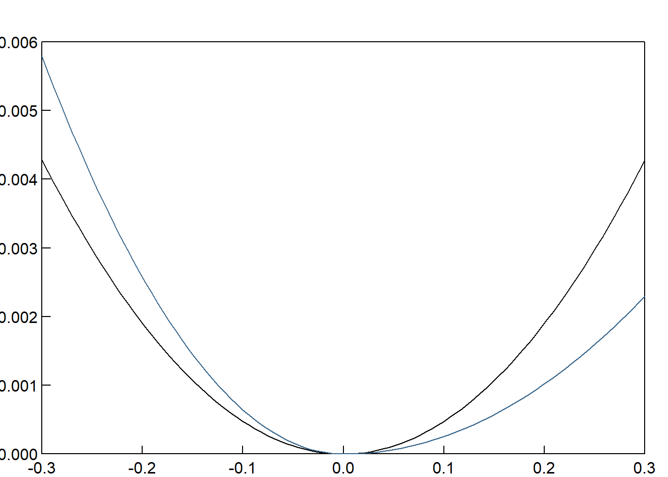
garch11.ni = newsimpact(garch11.fit)
gjrgarch11.ni = newsimpact(gjrgarch11.fit)
9.4 FIGURE 9.3. (Page 445)
News impact curves for S&P500 returns coefficients implied from GARCH and GJR model estimates
par(mfcol = c(1,1), oma = c(0,0,1,0) + 0.2, mar = c(0,1,0,0) + 1, mgp = c(0, 0.2, 0))
plot(garch11.ni$zx,garch11.ni$zy-min(abs(garch11.ni$zy)),type="l",las=1,xlab="",ylab="",main="",xaxs="i",yaxs="i",tck=.02,ylim=c(0,0.006))
lines(gjrgarch11.ni$zx,gjrgarch11.ni$zy-min(abs(gjrgarch11.ni$zy)),col="steelblue4")
9.5 GARCH-in-mean (Page 446)
garchm11.spec = ugarchspec(mean.model=list(armaOrder=c(0,0),archm=TRUE,archpow=1),
                           variance.model=list(garchOrder=c(1,1),model="sGARCH"))
garchm11.fit = ugarchfit(garchm11.spec,data=data$rjpy)
garchm11.fit
##
## *---------------------------------*
## *          GARCH Model Fit        *
## *---------------------------------*
##
## Conditional Variance Dynamics
## -----------------------------------
## GARCH Model  : sGARCH(1,1)
## Mean Model   : ARFIMA(0,0,0)
## Distribution : norm
##
## Optimal Parameters
## ------------------------------------
##         Estimate  Std. Error  t value Pr(>|t|)
## mu      0.024452    0.034364  0.71155 0.476743
## archm  -0.051739    0.079680 -0.64934 0.516121
## omega   0.004409    0.001117  3.94612 0.000079
## alpha1  0.047424    0.008052  5.88950 0.000000
## beta1   0.933047    0.011815 78.97247 0.000000
##
## Robust Standard Errors:
##         Estimate  Std. Error  t value Pr(>|t|)
## mu      0.024452    0.042288  0.57822 0.563115
## archm  -0.051739    0.095217 -0.54338 0.586870
## omega   0.004409    0.002816  1.56598 0.117352
## alpha1  0.047424    0.019557  2.42491 0.015312
## beta1   0.933047    0.028292 32.97891 0.000000
##
## LogLikelihood : -2460.776
##
## Information Criteria
## ------------------------------------
##
## Akaike       1.2369
## Bayes        1.2448
## Shibata      1.2369
## Hannan-Quinn 1.2397
##
## Weighted Ljung-Box Test on Standardized Residuals
## ------------------------------------
##                         statistic p-value
## Lag[1]                      102.7       0
## Lag[2*(p+q)+(p+q)-1][2]     103.8       0
## Lag[4*(p+q)+(p+q)-1][5]     107.0       0
## d.o.f=0
## H0 : No serial correlation
##
## Weighted Ljung-Box Test on Standardized Squared Residuals
## ------------------------------------
##                         statistic   p-value
## Lag[1]                      14.02 1.812e-04
## Lag[2*(p+q)+(p+q)-1][5]     18.07 6.541e-05
## Lag[4*(p+q)+(p+q)-1][9]     21.60 7.757e-05
## d.o.f=2
##
## Weighted ARCH LM Tests
## ------------------------------------
##             Statistic Shape Scale P-Value
## ARCH Lag[3]     3.478 0.500 2.000 0.06218
## ARCH Lag[5]     7.552 1.440 1.667 0.02571
## ARCH Lag[7]     9.400 2.315 1.543 0.02532
##
## Nyblom stability test
## ------------------------------------
## Joint Statistic:  0.7806
## Individual Statistics:
## mu     0.15261
## archm  0.15783
## omega  0.08669
## alpha1 0.09929
## beta1  0.12005
##
## Asymptotic Critical Values (10% 5% 1%)
## Joint Statistic:          1.28 1.47 1.88
## Individual Statistic:     0.35 0.47 0.75
##
## Sign Bias Test
## ------------------------------------
##                    t-value      prob sig
## Sign Bias           0.4557 6.486e-01
## Negative Sign Bias  4.6212 3.937e-06 ***
## Positive Sign Bias  1.8567 6.343e-02   *
## Joint Effect       30.2116 1.246e-06 ***
##
##
## Adjusted Pearson Goodness-of-Fit Test:
## ------------------------------------
##   group statistic p-value(g-1)
## 1    20     778.1   9.575e-153
## 2    30     969.4   2.481e-185
## 3    40    1156.7   3.103e-217
## 4    50    1252.4   4.850e-230
##
##
## Elapsed time : 0.678983
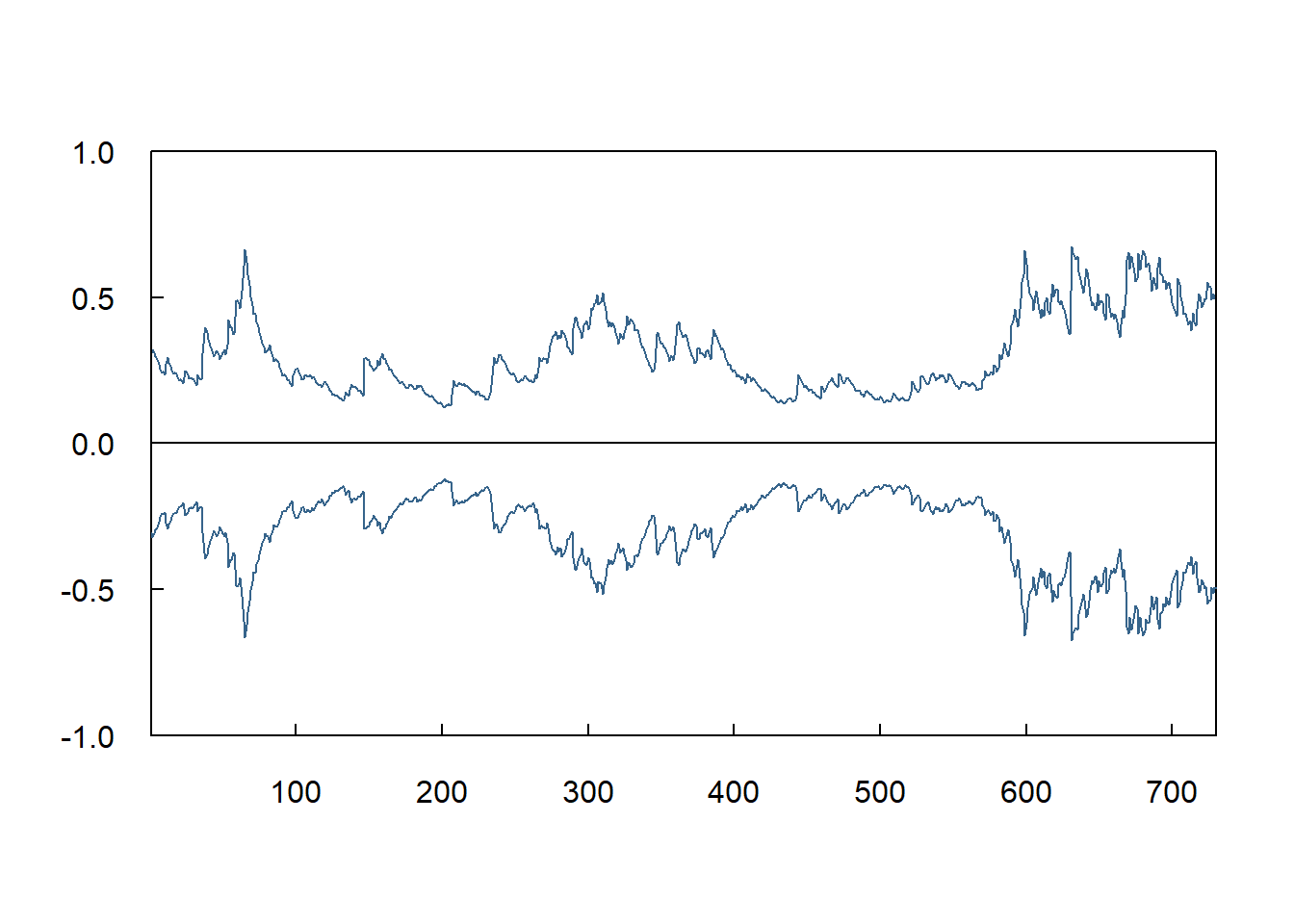
9.6 Screenshot 9.4 Dynamic forecasts of the conditional variance (Page 450)
egarch11.fore = ugarchforecast(egarch11.fit,n.ahead=730)
lower =-1.65*egarch11.fore@forecast$sigmaFor
upper = 1.65*egarch11.fore@forecast$sigmaFor
plot(lower,type="l",las=1,xlab="",ylab="",main="",xaxs="i",yaxs="i",tck=.02,ylim=c(-1,1),col="steelblue4")
lines(upper,col="steelblue4")
abline(h=0)
9.7 Screenshot 9.5 Static forecasts of the conditional variance (Page 451)
library(xts)

# Ensure 'data' has a Date column
rjpy_xts <- xts(data$rjpy, order.by = data$Date)

space <- 730
sigma.fore <- numeric(space)

for (i in 1:space) {
   dynamic.egarch.fit <- ugarchfit(egarch11.spec, rjpy_xts[1:(nrow(rjpy_xts)-space+i)])
   sigma.fore[i] <- ugarchforecast(dynamic.egarch.fit, n.ahead = 1)@forecast$sigmaFor
   if (i %% 50 == 0) {
      print(i / space * 100)
   }
}
## [1] 6.849315
## [1] 13.69863
## [1] 20.54795
## [1] 27.39726
## [1] 34.24658
## [1] 41.09589
## [1] 47.94521
## [1] 54.79452
## [1] 61.64384
## [1] 68.49315
## [1] 75.34247
## [1] 82.19178
## [1] 89.0411
## [1] 95.89041
plot(2 * sigma.fore^2, type = "l", las = 1, xlab = "", ylab = "",
     main = "", xaxs = "i", yaxs = "i", tck = .02, col = "steelblue4", ylim = c(-1, 1))
lines(-2 * sigma.fore^2, col = "steelblue4")
abline(h = 0)