Testing for unit roots (Page 371)
library("foreign")
data = read.dta("Dataset/ukhp.dta")

library("urca")
df.hp = ur.df(data$HP,type="drift",lags=2)
df.hp@testreg
##
## Call:
## lm(formula = z.diff ~ z.lag.1 + 1 + z.diff.lag)
##
## Residuals:
##     Min      1Q  Median      3Q     Max
## -4825.5  -618.4   -22.6   629.0  4787.3
##
## Coefficients:
##               Estimate Std. Error t value Pr(>|t|)
## (Intercept)  2.345e+02  1.768e+02   1.326    0.186
## z.lag.1     -6.858e-04  1.458e-03  -0.470    0.639
## z.diff.lag1  3.162e-01  5.837e-02   5.417 1.37e-07 ***
## z.diff.lag2  3.332e-01  5.840e-02   5.706 3.12e-08 ***
## ---
## Signif. codes:  0 '***' 0.001 '**' 0.01 '*' 0.05 '.' 0.1 ' ' 1
##
## Residual standard error: 1187 on 262 degrees of freedom
## Multiple R-squared:  0.3086, Adjusted R-squared:  0.3007
## F-statistic: 38.98 on 3 and 262 DF,  p-value: < 2.2e-16
Testing for unit roots (Page 372)
df.dhp = ur.df(diff(data$HP),type="drift",lags=1)
df.dhp@testreg
##
## Call:
## lm(formula = z.diff ~ z.lag.1 + 1 + z.diff.lag)
##
## Residuals:
##     Min      1Q  Median      3Q     Max
## -4873.3  -595.6   -15.6   632.7  4759.0
##
## Coefficients:
##              Estimate Std. Error t value Pr(>|t|)
## (Intercept) 159.66720   76.90883   2.076   0.0389 *
## z.lag.1      -0.35126    0.05996  -5.858 1.40e-08 ***
## z.diff.lag   -0.33262    0.05830  -5.706 3.12e-08 ***
## ---
## Signif. codes:  0 '***' 0.001 '**' 0.01 '*' 0.05 '.' 0.1 ' ' 1
##
## Residual standard error: 1185 on 263 degrees of freedom
## Multiple R-squared:  0.3437, Adjusted R-squared:  0.3387
## F-statistic: 68.87 on 2 and 263 DF,  p-value: < 2.2e-16
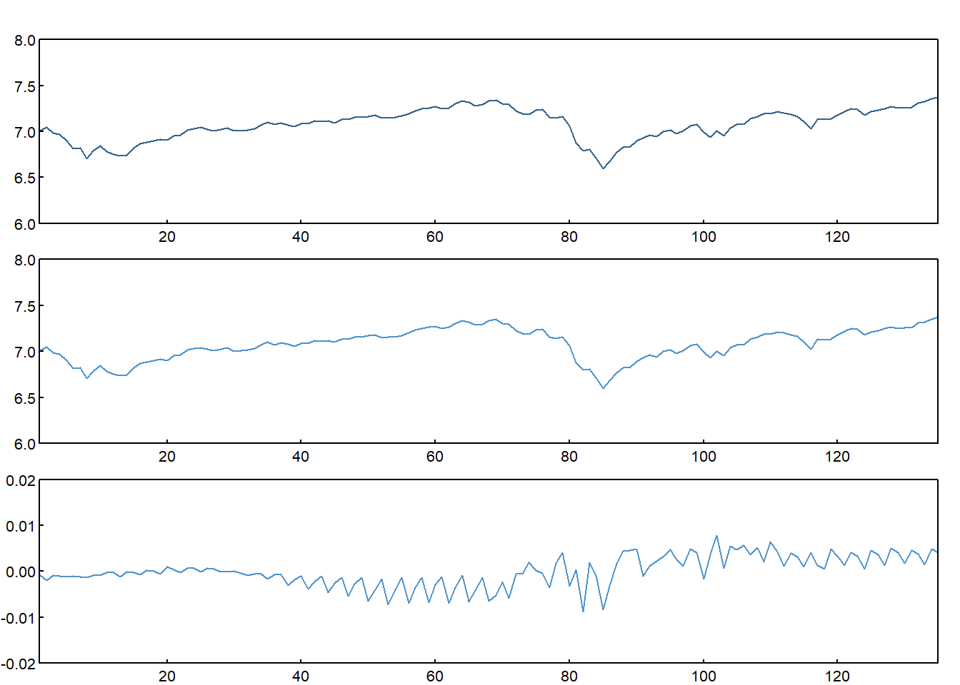
Screenshot 8.2 Actual, fitted and residual plot to check for stationarity (Page 401)
data = read.dta("Dataset/SandPhedge.dta")

lm1 = lm(lspot~lfutures,data=data)
summary(lm1)
##
## Call:
## lm(formula = lspot ~ lfutures, data = data)
##
## Residuals:
##        Min         1Q     Median         3Q        Max
## -0.0088008 -0.0014023 -0.0003198  0.0021394  0.0077902
##
## Coefficients:
##             Estimate Std. Error t value Pr(>|t|)
## (Intercept) 0.025310   0.012061   2.099   0.0377 *
## lfutures    0.996468   0.001704 584.661   <2e-16 ***
## ---
## Signif. codes:  0 '***' 0.001 '**' 0.01 '*' 0.05 '.' 0.1 ' ' 1
##
## Residual standard error: 0.003362 on 133 degrees of freedom
## Multiple R-squared:  0.9996, Adjusted R-squared:  0.9996
## F-statistic: 3.418e+05 on 1 and 133 DF,  p-value: < 2.2e-16
par(mfcol = c(3,1), oma = c(0,0,1,0) + 0.2, mar = c(0,1,0,0) + 1, mgp = c(0, 0.2, 0))
plot(data$lspot,type="l",las=1,xlab="",ylab="",main="",xaxs="i",yaxs="i",tck=.02,col="steelblue4",ylim=c(6,8))
plot(lm1$fitted.values,type="l",las=1,xlab="",ylab="",main="",xaxs="i",yaxs="i",tck=.02,col="steelblue3",ylim=c(6,8))
plot(lm1$residuals,type="l",las=1,xlab="",ylab="",main="",xaxs="i",yaxs="i",tck=.02,col="steelblue3",ylim=c(-0.02,0.02))
Testing for cointegration (Page 402)
df.res = ur.df(lm1$residuals,lags=2,type="drift")
df.res@testreg
##
## Call:
## lm(formula = z.diff ~ z.lag.1 + 1 + z.diff.lag)
##
## Residuals:
##        Min         1Q     Median         3Q        Max
## -0.0109049 -0.0007591 -0.0001212  0.0007334  0.0089030
##
## Coefficients:
##               Estimate Std. Error t value Pr(>|t|)
## (Intercept)  7.969e-05  1.934e-04   0.412   0.6810
## z.lag.1     -1.202e-01  6.913e-02  -1.738   0.0845 .
## z.diff.lag1 -6.589e-01  8.389e-02  -7.854 1.42e-12 ***
## z.diff.lag2 -5.582e-01  7.428e-02  -7.514 8.71e-12 ***
## ---
## Signif. codes:  0 '***' 0.001 '**' 0.01 '*' 0.05 '.' 0.1 ' ' 1
##
## Residual standard error: 0.002221 on 128 degrees of freedom
## Multiple R-squared:  0.5061, Adjusted R-squared:  0.4946
## F-statistic: 43.73 on 3 and 128 DF,  p-value: < 2.2e-16
Cointegration Test (Page 406)
data = read.dta("Dataset/macro.dta")

df = data.frame(data$USTB10Y,data$USTB1Y,data$USTB3M,data$USTB3Y,data$USTB5Y,data$USTB6M)
p=3
jo.ci.trace = ca.jo(df,type="trace",ecdet="const",K=p+1)
summary(jo.ci.trace)
##
## ######################
## # Johansen-Procedure #
## ######################
##
## Test type: trace statistic , without linear trend and constant in cointegration
##
## Eigenvalues (lambda):
## [1] 1.373725e-01 1.185885e-01 8.964990e-02 4.634717e-02 2.483427e-02 7.987276e-03 8.153200e-17
##
## Values of teststatistic and critical values of test:
##
##            test 10pct   5pct   1pct
## r <= 5 |   2.58  7.52   9.24  12.97
## r <= 4 |  10.68 17.85  19.96  24.60
## r <= 3 |  25.96 32.00  34.91  41.07
## r <= 2 |  56.20 49.65  53.12  60.16
## r <= 1 |  96.85 71.86  76.07  84.45
## r = 0  | 144.43 97.18 102.14 111.01
##
## Eigenvectors, normalised to first column:
## (These are the cointegration relations)
##
##                 data.USTB10Y.l4 data.USTB1Y.l4 data.USTB3M.l4 data.USTB3Y.l4 data.USTB5Y.l4
## data.USTB10Y.l4       1.0000000       1.000000      1.0000000      1.0000000     1.00000000
## data.USTB1Y.l4       -6.7348169      -5.852282     -2.9674724      0.9370732    -0.06084815
## data.USTB3M.l4       -4.5669473       0.751493      2.5491180      0.2850950    -0.06281291
## data.USTB3Y.l4        4.0561742     -17.238836      5.4836484      0.9824287     0.54586734
## data.USTB5Y.l4       -3.2821195      11.470920     -4.5162308     -2.1913592    -1.42474873
## data.USTB6M.l4        9.4830397      11.048983     -1.6063534     -0.9661132     0.06560961
## constant             -0.4412386      -5.257480      0.4937381     -0.2650234    -0.69346419
##                 data.USTB6M.l4    constant
## data.USTB10Y.l4     1.00000000  1.00000000
## data.USTB1Y.l4     -0.09406147  0.37329716
## data.USTB3M.l4     -0.12530350 -0.58224116
## data.USTB3Y.l4      0.54989363  3.51288142
## data.USTB5Y.l4     -1.20164104 -4.71131952
## data.USTB6M.l4      0.18999602 -0.06925111
## constant           -1.61396696  3.92524749
##
## Weights W:
## (This is the loading matrix)
##
##                data.USTB10Y.l4 data.USTB1Y.l4 data.USTB3M.l4 data.USTB3Y.l4 data.USTB5Y.l4
## data.USTB10Y.d      0.05690502   -0.005886205     0.08166862     0.12974599     0.02429021
## data.USTB1Y.d       0.06011374   -0.013113342     0.03704386     0.04221975     0.12632957
## data.USTB3M.d       0.08534176   -0.021186294    -0.02974528     0.04163139     0.08187311
## data.USTB3Y.d       0.04302183   -0.005157639     0.03880503     0.13379182     0.11657737
## data.USTB5Y.d       0.05752479   -0.004287452     0.07114089     0.16726624     0.08141523
## data.USTB6M.d       0.03958347   -0.020450550     0.01672614     0.04243206     0.10327850
##                data.USTB6M.l4      constant
## data.USTB10Y.d   -0.028240500  1.074784e-15
## data.USTB1Y.d    -0.017173146 -2.794624e-15
## data.USTB3M.d    -0.007619134 -3.291100e-15
## data.USTB3Y.d    -0.027423330  1.036733e-15
## data.USTB5Y.d    -0.026315900  1.840829e-15
## data.USTB6M.d    -0.011131403 -1.856540e-15
Johansen System Cointegration Test (Page 407)
jo.ci.eigen = ca.jo(df,type="trace",ecdet="const",K=p+1)
summary(jo.ci.eigen)
##
## ######################
## # Johansen-Procedure #
## ######################
##
## Test type: trace statistic , without linear trend and constant in cointegration
##
## Eigenvalues (lambda):
## [1] 1.373725e-01 1.185885e-01 8.964990e-02 4.634717e-02 2.483427e-02 7.987276e-03 8.153200e-17
##
## Values of teststatistic and critical values of test:
##
##            test 10pct   5pct   1pct
## r <= 5 |   2.58  7.52   9.24  12.97
## r <= 4 |  10.68 17.85  19.96  24.60
## r <= 3 |  25.96 32.00  34.91  41.07
## r <= 2 |  56.20 49.65  53.12  60.16
## r <= 1 |  96.85 71.86  76.07  84.45
## r = 0  | 144.43 97.18 102.14 111.01
##
## Eigenvectors, normalised to first column:
## (These are the cointegration relations)
##
##                 data.USTB10Y.l4 data.USTB1Y.l4 data.USTB3M.l4 data.USTB3Y.l4 data.USTB5Y.l4
## data.USTB10Y.l4       1.0000000       1.000000      1.0000000      1.0000000     1.00000000
## data.USTB1Y.l4       -6.7348169      -5.852282     -2.9674724      0.9370732    -0.06084815
## data.USTB3M.l4       -4.5669473       0.751493      2.5491180      0.2850950    -0.06281291
## data.USTB3Y.l4        4.0561742     -17.238836      5.4836484      0.9824287     0.54586734
## data.USTB5Y.l4       -3.2821195      11.470920     -4.5162308     -2.1913592    -1.42474873
## data.USTB6M.l4        9.4830397      11.048983     -1.6063534     -0.9661132     0.06560961
## constant             -0.4412386      -5.257480      0.4937381     -0.2650234    -0.69346419
##                 data.USTB6M.l4    constant
## data.USTB10Y.l4     1.00000000  1.00000000
## data.USTB1Y.l4     -0.09406147  0.37329716
## data.USTB3M.l4     -0.12530350 -0.58224116
## data.USTB3Y.l4      0.54989363  3.51288142
## data.USTB5Y.l4     -1.20164104 -4.71131952
## data.USTB6M.l4      0.18999602 -0.06925111
## constant           -1.61396696  3.92524749
##
## Weights W:
## (This is the loading matrix)
##
##                data.USTB10Y.l4 data.USTB1Y.l4 data.USTB3M.l4 data.USTB3Y.l4 data.USTB5Y.l4
## data.USTB10Y.d      0.05690502   -0.005886205     0.08166862     0.12974599     0.02429021
## data.USTB1Y.d       0.06011374   -0.013113342     0.03704386     0.04221975     0.12632957
## data.USTB3M.d       0.08534176   -0.021186294    -0.02974528     0.04163139     0.08187311
## data.USTB3Y.d       0.04302183   -0.005157639     0.03880503     0.13379182     0.11657737
## data.USTB5Y.d       0.05752479   -0.004287452     0.07114089     0.16726624     0.08141523
## data.USTB6M.d       0.03958347   -0.020450550     0.01672614     0.04243206     0.10327850
##                data.USTB6M.l4      constant
## data.USTB10Y.d   -0.028240500  1.074784e-15
## data.USTB1Y.d    -0.017173146 -2.794624e-15
## data.USTB3M.d    -0.007619134 -3.291100e-15
## data.USTB3Y.d    -0.027423330  1.036733e-15
## data.USTB5Y.d    -0.026315900  1.840829e-15
## data.USTB6M.d    -0.011131403 -1.856540e-15
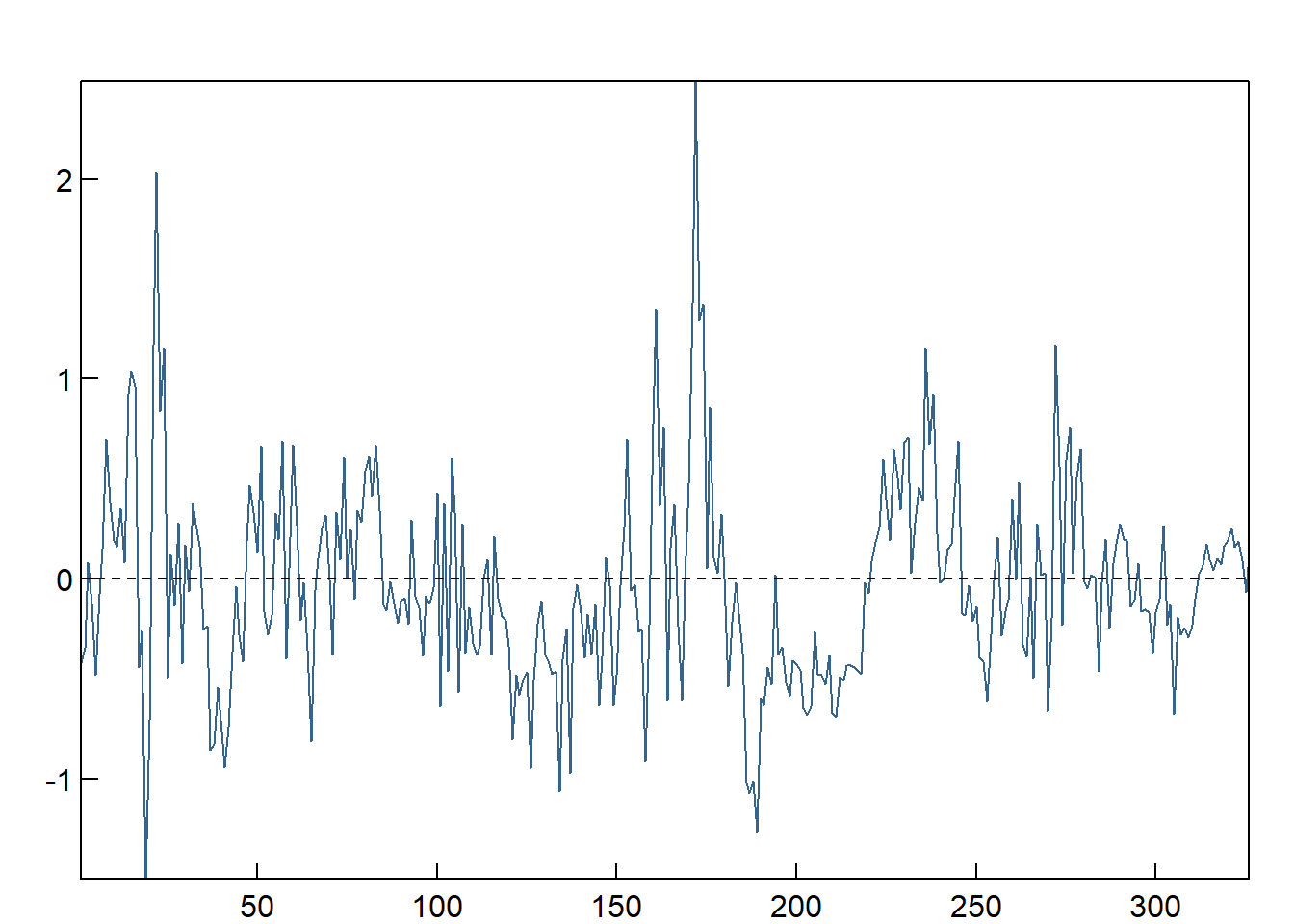
ECM = cbind(as.matrix(df),1)%*%jo.ci.eigen@V[,1]

par(mfcol = c(1,1), oma = c(0,0,1,0) + 0.2, mar = c(0,1,0,0) + 1, mgp = c(0, 0.2, 0))
plot(ECM,type="l",las=1,xlab="",ylab="",main="",xaxs="i",yaxs="i",tck=.02,col="steelblue4")
abline(h=0,lty=2)