Screenshot 3.2. Summary statistics for spot and futures (Page 88)
library(foreign)
library(moments)

data_sp <- read.dta("Dataset/SandPhedge.dta")
data_sp$Date <- seq(2002 + 2/12, 2013 + 4/12, by = 1/12)
data_sp <- na.omit(data_sp)

Y <- cbind(rspot = data_sp$rspot, rfutures = data_sp$rfutures)
summary_stats <- data.frame(
  Mean = apply(Y, 2, mean),
  Median = apply(Y, 2, median),
  Max = apply(Y, 2, max),
  Min = apply(Y, 2, min),
  SD = apply(Y, 2, sd),
  Skewness = apply(Y, 2, skewness),
  Kurtosis = apply(Y, 2, kurtosis)
)

jarque_tests <- lapply(1:2, function(i) jarque.test(Y[, i]))
names(jarque_tests) <- colnames(Y)

summary_stats
##               Mean   Median      Max       Min       SD   Skewness Kurtosis
## rspot    0.2739265 1.101731 10.06554 -18.38397 4.591529 -0.9111043 4.740732
## rfutures 0.2713085 1.024841 10.39119 -18.80256 4.548128 -0.9275250 4.878594
## $rspot
##
##  Jarque-Bera Normality Test
##
## data:  Y[, i]
## JB = 35.457, p-value = 1.998e-08
## alternative hypothesis: greater
##
##
## $rfutures
##
##  Jarque-Bera Normality Test
##
## data:  Y[, i]
## JB = 38.918, p-value = 3.541e-09
## alternative hypothesis: greater
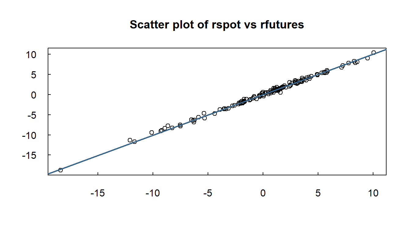
Screenshot 3.4 Regression Estimation results (Page 90)
plot(Y, type = "p", las = 1, xlab = "", ylab = "", main = "Scatter plot of rspot vs rfutures", tck = 0.02)
lm_sp <- lm(rspot ~ rfutures, data = data_sp)
abline(lm_sp, col = "steelblue4", lwd = 2)
CAPM Data Prep (Page 123)
data_capm <- read.dta("Dataset/capm.dta")
data_capm$Date <- seq(2002 + 1/12, 2013 + 4/12, by = 1/12)

rsandp <- 100 * diff(log(data_capm$SANDP))
rford <- 100 * diff(log(data_capm$FORD))
ustb3m <- data_capm$USTB3M[-1] / 12

# Excess returns
erford <- rford - ustb3m
ersandp <- rsandp - ustb3m
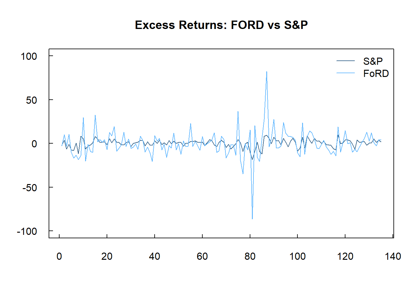
Screenshot 3.5 Plot of the two series (PP 125)
# Plot the first series
plot(ersandp, type = "l", las = 1, col = "steelblue4",
     main = "Excess Returns: FORD vs S&P", xlab = "", ylab = "", ylim = c(-100, 100), tck = 0.02)

# Add the second series
lines(erford, type = "l", col = "steelblue1")

legend("topright", legend = c("S&P", "FoRD"),
       col = c("steelblue4", "steelblue1"), lty = 1, bty = "n")
CAPM Regression Table (Page 126)
summary(lm_capm <- lm(erford ~ ersandp))
##
## Call:
## lm(formula = erford ~ ersandp)
##
## Residuals:
##     Min      1Q  Median      3Q     Max
## -48.797  -7.294  -1.225   5.593  63.461
##
## Coefficients:
##             Estimate Std. Error t value Pr(>|t|)
## (Intercept)  -0.4475     1.0886  -0.411    0.682
## ersandp       2.0208     0.2383   8.481 3.76e-14 ***
## ---
## Signif. codes:  0 '***' 0.001 '**' 0.01 '*' 0.05 '.' 0.1 ' ' 1
##
## Residual standard error: 12.63 on 133 degrees of freedom
## Multiple R-squared:  0.351,  Adjusted R-squared:  0.3461
## F-statistic: 71.93 on 1 and 133 DF,  p-value: 3.758e-14