Testing for heteroscedasticity (Page 187)
# First regression
lm1 <- lm(ermsoft ~ ersandp + dprod + dcredit + dinflation + dmoney + dspread + rterm, data = data)

# Add residuals squared to data frame
data$Resid = lm1$residuals
data$Resid_sq <- resid(lm1)^2

# Second regression using squared predictors
lm2 <- lm(Resid_sq ~ I(ersandp^2) + I(dprod^2) + I(dcredit^2) +
            I(dinflation^2) + I(dmoney^2) + I(dspread^2) + I(rterm^2),
          data = data)

# Display summary
summary(lm2)
##
## Call:
## lm(formula = Resid_sq ~ I(ersandp^2) + I(dprod^2) + I(dcredit^2) +
##     I(dinflation^2) + I(dmoney^2) + I(dspread^2) + I(rterm^2),
##     data = data)
##
## Residuals:
##    Min     1Q Median     3Q    Max
## -188.9 -159.1 -129.7  -68.2 4305.1
##
## Coefficients:
##                   Estimate Std. Error t value Pr(>|t|)
## (Intercept)      1.936e+02  4.283e+01   4.519 8.79e-06 ***
## I(ersandp^2)    -1.627e-01  6.984e-01  -0.233    0.816
## I(dprod^2)      -1.134e+01  3.119e+01  -0.363    0.717
## I(dcredit^2)    -1.013e-08  3.983e-08  -0.254    0.799
## I(dinflation^2) -6.578e+01  1.500e+02  -0.438    0.661
## I(dmoney^2)     -1.228e-02  2.722e-02  -0.451    0.652
## I(dspread^2)    -2.023e+00  6.384e+02  -0.003    0.997
## I(rterm^2)      -1.963e+02  2.944e+02  -0.667    0.505
## ---
## Signif. codes:  0 '***' 0.001 '**' 0.01 '*' 0.05 '.' 0.1 ' ' 1
##
## Residual standard error: 558.5 on 316 degrees of freedom
## Multiple R-squared:  0.006295,   Adjusted R-squared:  -0.01572
## F-statistic: 0.286 on 7 and 316 DF,  p-value: 0.9592
The Breusch–Godfrey test or Autocorrelation (pp208)
p <- 10
Reslag <- embed(data$Resid, p + 1)[, -1]
lm3 <- lm(Resid ~ ersandp + dprod + dcredit + dinflation + dmoney + dspread + rterm + Reslag,
          data = data[-(1:p), ])
summary(lm3)
##
## Call:
## lm(formula = Resid ~ ersandp + dprod + dcredit + dinflation +
##     dmoney + dspread + rterm + Reslag, data = data[-(1:p), ])
##
## Residuals:
##     Min      1Q  Median      3Q     Max
## -62.962  -3.806   1.031   6.066  27.327
##
## Coefficients:
##               Estimate Std. Error t value Pr(>|t|)
## (Intercept) -2.574e-01  8.898e-01  -0.289  0.77257
## ersandp     -4.231e-02  1.580e-01  -0.268  0.78908
## dprod        6.400e-02  1.296e+00   0.049  0.96064
## dcredit      1.752e-06  7.485e-05   0.023  0.98134
## dinflation  -4.591e-01  2.181e+00  -0.211  0.83340
## dmoney      -4.422e-03  3.447e-02  -0.128  0.89800
## dspread      1.530e+00  6.851e+00   0.223  0.82348
## rterm        7.962e-01  2.523e+00   0.316  0.75257
## Reslag1     -1.647e-01  5.847e-02  -2.817  0.00517 **
## Reslag2     -8.471e-02  5.805e-02  -1.459  0.14552
## Reslag3     -4.682e-02  5.797e-02  -0.808  0.41994
## Reslag4     -1.387e-01  5.725e-02  -2.423  0.01601 *
## Reslag5     -1.255e-01  5.654e-02  -2.220  0.02720 *
## Reslag6     -1.138e-01  5.645e-02  -2.016  0.04466 *
## Reslag7     -7.230e-02  5.675e-02  -1.274  0.20363
## Reslag8     -1.123e-01  5.668e-02  -1.982  0.04842 *
## Reslag9     -1.632e-01  5.678e-02  -2.874  0.00435 **
## Reslag10    -6.171e-02  5.690e-02  -1.085  0.27895
## ---
## Signif. codes:  0 '***' 0.001 '**' 0.01 '*' 0.05 '.' 0.1 ' ' 1
##
## Residual standard error: 12.26 on 296 degrees of freedom
## Multiple R-squared:  0.07896,    Adjusted R-squared:  0.02606
## F-statistic: 1.493 on 17 and 296 DF,  p-value: 0.09573
Screenshot 5.2 Non-normality test results (Page 211)
par(mfcol = c(1, 1), oma = c(0.2, 0.2, 1.2, 0.2), mar = c(1, 2, 1, 1), mgp = c(0, 0.2, 0))
hist(data$Resid, freq = TRUE, breaks = 40, las = 1, col = "steelblue4",
     xlab = "", ylab = "", main = "", xaxs = "i", yaxs = "i", xlim = c(-70, 30), tck = 0.02)
box()
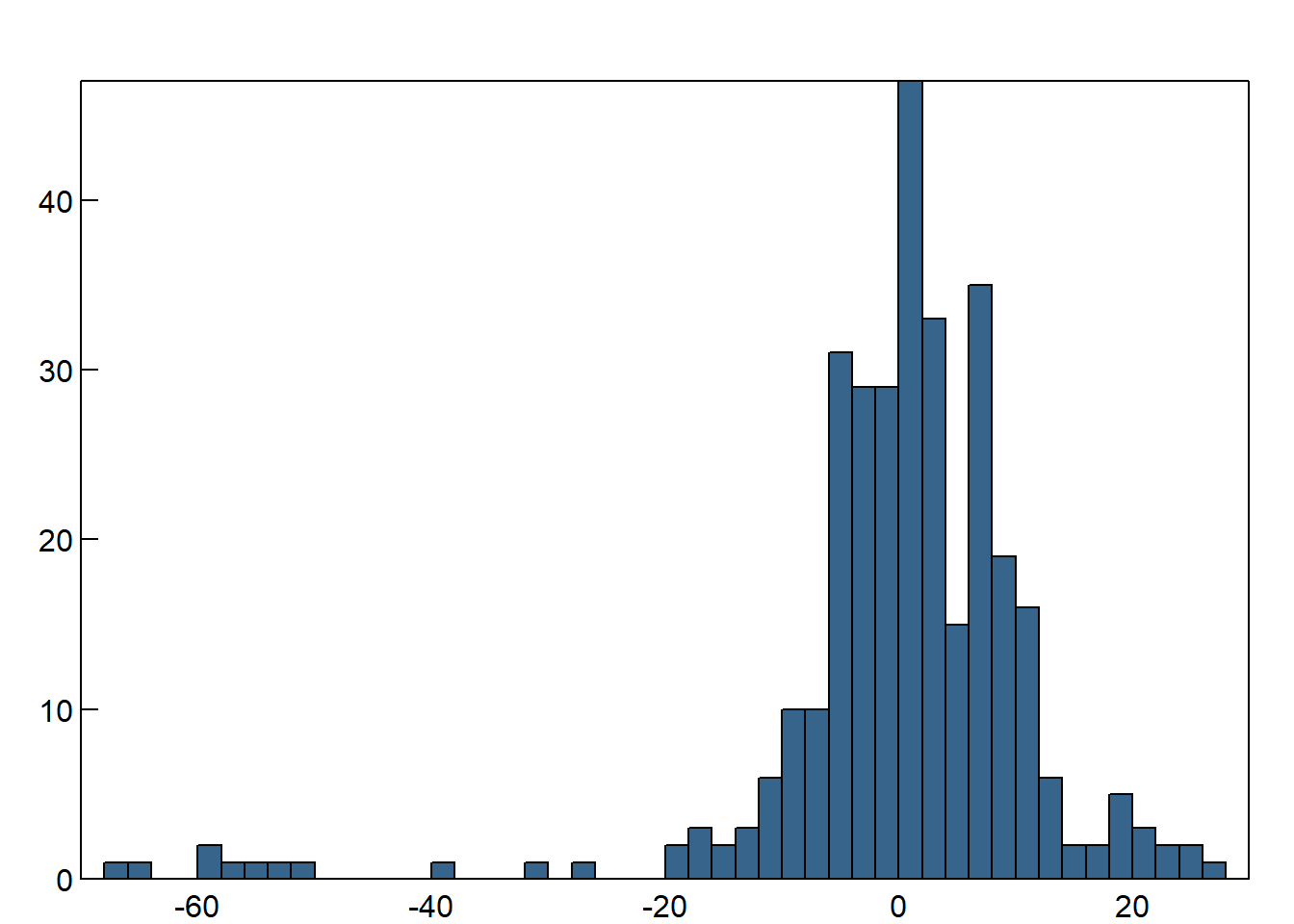
##    Min. 1st Qu.  Median    Mean 3rd Qu.    Max.
## -66.985  -3.643   1.105   0.000   6.661  26.587
## [1] 12.5209
library(moments)
skewness(data$Resid)
## [1] -2.535283
## [1] 13.53493
##
##  Jarque-Bera Normality Test
##
## data:  data$Resid
## JB = 1845.4, p-value < 2.2e-16
## alternative hypothesis: greater
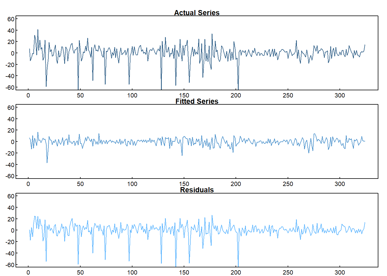
Screenshot 5.3 Regression residuals, actual values and fitted series (Page 215)
par(mfcol = c(3, 1), oma = c(0.2, 0.2, 1.2, 0.2), mar = c(1, 2, 1, 1), mgp = c(0, 0.2, 0))
plot(data$ermsoft, type = "l", las = 1, col = "steelblue4", main = "Actual Series",
     xlab = "", ylab = "", ylim = c(-60, 60), tck = 0.02)
plot(fitted(lm1), type = "l", las = 1, col = "steelblue3", main = "Fitted Series",
     xlab = "", ylab = "", ylim = c(-60, 60), tck = 0.02)
plot(data$Resid, type = "l", las = 1, col = "steelblue1", main = "Residuals",
     xlab = "", ylab = "", ylim = c(-60, 60), tck = 0.02)
Regression with Dummy Variables (Page 216)
lm4 <- lm(ermsoft ~ ersandp + dprod + dcredit + dinflation + dmoney + dspread + rterm + FEB98DUM + FEB03DUM,
          data = data)
summary(lm4)
##
## Call:
## lm(formula = ermsoft ~ ersandp + dprod + dcredit + dinflation +
##     dmoney + dspread + rterm + FEB98DUM + FEB03DUM, data = data)
##
## Residuals:
##     Min      1Q  Median      3Q     Max
## -59.475  -4.229   0.650   6.434  25.494
##
## Coefficients:
##               Estimate Std. Error t value Pr(>|t|)
## (Intercept)  2.941e-01  8.262e-01   0.356   0.7221
## ersandp      1.401e+00  1.432e-01   9.787  < 2e-16 ***
## dprod       -1.334e+00  1.207e+00  -1.105   0.2699
## dcredit     -3.948e-05  6.962e-05  -0.567   0.5711
## dinflation   3.518e+00  1.975e+00   1.781   0.0759 .
## dmoney      -2.196e-02  3.210e-02  -0.684   0.4944
## dspread      5.351e+00  6.302e+00   0.849   0.3965
## rterm        4.650e+00  2.291e+00   2.029   0.0433 *
## FEB98DUM    -6.648e+01  1.160e+01  -5.729 2.37e-08 ***
## FEB03DUM    -6.761e+01  1.158e+01  -5.838 1.32e-08 ***
## ---
## Signif. codes:  0 '***' 0.001 '**' 0.01 '*' 0.05 '.' 0.1 ' ' 1
##
## Residual standard error: 11.53 on 314 degrees of freedom
## Multiple R-squared:  0.3461, Adjusted R-squared:  0.3273
## F-statistic: 18.46 on 9 and 314 DF,  p-value: < 2.2e-16
Correlation Matrix (Page 220)
df <- data[, c("dprod", "dcredit", "dinflation", "dmoney", "dspread", "rterm")]
cor(df)
##                   dprod      dcredit  dinflation      dmoney      dspread        rterm
## dprod       1.000000000  0.141066050 -0.12426873 -0.13006021 -0.055572949 -0.002375089
## dcredit     0.141066050  1.000000000  0.04516382 -0.01172447  0.015264080  0.009675069
## dinflation -0.124268730  0.045163824  1.00000000 -0.09797243 -0.224837965 -0.054192265
## dmoney     -0.130060210 -0.011724472 -0.09797243  1.00000000  0.213575550 -0.086217900
## dspread    -0.055572949  0.015264080 -0.22483797  0.21357555  1.000000000  0.001570935
## rterm      -0.002375089  0.009675069 -0.05419227 -0.08621790  0.001570935  1.000000000
RESET Test (Page 224)
lm5 <- lm(ermsoft ~ ersandp + dprod + dcredit + dinflation + dmoney + dspread + rterm + FEB98DUM + FEB03DUM + I(fitted(lm4)^2),
          data = data)
summary(lm5)
##
## Call:
## lm(formula = ermsoft ~ ersandp + dprod + dcredit + dinflation +
##     dmoney + dspread + rterm + FEB98DUM + FEB03DUM + I(fitted(lm4)^2),
##     data = data)
##
## Residuals:
##     Min      1Q  Median      3Q     Max
## -58.928  -4.298   0.943   6.322  24.747
##
## Coefficients:
##                    Estimate Std. Error t value Pr(>|t|)
## (Intercept)      -2.838e-01  8.934e-01  -0.318 0.750997
## ersandp           1.500e+00  1.545e-01   9.709  < 2e-16 ***
## dprod            -1.447e+00  1.205e+00  -1.201 0.230702
## dcredit          -3.078e-05  6.962e-05  -0.442 0.658686
## dinflation        3.586e+00  1.970e+00   1.820 0.069663 .
## dmoney           -2.251e-02  3.201e-02  -0.703 0.482480
## dspread           4.487e+00  6.305e+00   0.712 0.477196
## rterm             4.518e+00  2.286e+00   1.976 0.049030 *
## FEB98DUM         -1.046e+02  2.557e+01  -4.091 5.46e-05 ***
## FEB03DUM         -1.236e+02  3.544e+01  -3.489 0.000555 ***
## I(fitted(lm4)^2)  1.172e-02  7.007e-03   1.672 0.095478 .
## ---
## Signif. codes:  0 '***' 0.001 '**' 0.01 '*' 0.05 '.' 0.1 ' ' 1
##
## Residual standard error: 11.5 on 313 degrees of freedom
## Multiple R-squared:  0.3518, Adjusted R-squared:  0.3311
## F-statistic: 16.99 on 10 and 313 DF,  p-value: < 2.2e-16
library(lmtest)
reset(lm4, power = 2)
##
##  RESET test
##
## data:  lm4
## RESET = 2.7964, df1 = 1, df2 = 313, p-value = 0.09548