Estimating the inflation equation (Page 325)
library("foreign")
data = read.dta("Dataset/macro.dta")
data = na.omit(data)

library("systemfit")
eq1 = data$inflation ~ data$dprod + data$dcredit + data$dmoney + data$rsandp
eq2 = data$rsandp ~ data$dprod + data$dspread + data$rterm + data$inflation

inst = ~ income + farmPrice + trend
eqSystem = list(eq1, eq2)
SEM = systemfit(eqSystem,method="SUR")
SEM$eq[[1]]$coefficients
##   (Intercept)    data$dprod  data$dcredit   data$dmoney   data$rsandp
##  2.505916e-01 -1.258143e-02  1.512073e-06 -4.161894e-03  1.702656e-04
##    (Intercept)     data$dprod   data$dspread     data$rterm data$inflation
##      0.8417346     -0.2741500     -8.4161465     -0.3354731     -0.9654215
library(foreign)
library(systemfit)

data <- na.omit(read.dta("Dataset/macro.dta"))

eqSystem <- list(
  inflation ~ dprod + dcredit + dmoney + rsandp,
  rsandp ~ dprod + dspread + rterm + inflation
)

inst <- ~ income + farmPrice + trend

SEM <- systemfit(eqSystem, method = "SUR", inst = inst, data = data)

#SUR estimates for 'eq1' (equation 1)
SEM$eq[[1]]$coefficients
##   (Intercept)         dprod       dcredit        dmoney        rsandp
##  2.505916e-01 -1.258143e-02  1.512073e-06 -4.161894e-03  1.702656e-04
# SUR estimates for 'eq2' (equation 2)
SEM$eq[[2]]$coefficients
## (Intercept)       dprod     dspread       rterm   inflation
##   0.8417346  -0.2741500  -8.4161465  -0.3354731  -0.9654215
VAR estimation (Page 345)
data = read.dta("Dataset/currencies.dta")
data = na.omit(data)

library("vars")
Y = data.frame(reur=data$reur,rgbp=data$rgbp,rjpy=data$rjpy)
VAR.cur = VAR(Y,p=2)
summary(VAR.cur)
##
## VAR Estimation Results:
## =========================
## Endogenous variables: reur, rgbp, rjpy
## Deterministic variables: const
## Sample size: 3985
## Log Likelihood: -6043.54
## Roots of the characteristic polynomial:
## 0.3329 0.3329 0.1532 0.1146 0.1146 0.002806
## Call:
## VAR(y = Y, p = 2)
##
##
## Estimation results for equation reur:
## =====================================
## reur = reur.l1 + rgbp.l1 + rjpy.l1 + reur.l2 + rgbp.l2 + rjpy.l2 + const
##
##          Estimate Std. Error t value Pr(>|t|)
## reur.l1  0.200155   0.022708   8.814   <2e-16 ***
## rgbp.l1 -0.061566   0.024107  -2.554   0.0107 *
## rjpy.l1 -0.020151   0.016658  -1.210   0.2265
## reur.l2 -0.033413   0.022619  -1.477   0.1397
## rgbp.l2  0.024656   0.024079   1.024   0.3059
## rjpy.l2  0.002628   0.016682   0.158   0.8748
## const   -0.005836   0.007453  -0.783   0.4337
## ---
## Signif. codes:  0 '***' 0.001 '**' 0.01 '*' 0.05 '.' 0.1 ' ' 1
##
##
## Residual standard error: 0.4703 on 3978 degrees of freedom
## Multiple R-Squared: 0.02548, Adjusted R-squared: 0.02401
## F-statistic: 17.33 on 6 and 3978 DF,  p-value: < 2.2e-16
##
##
## Estimation results for equation rgbp:
## =====================================
## rgbp = reur.l1 + rgbp.l1 + rjpy.l1 + reur.l2 + rgbp.l2 + rjpy.l2 + const
##
##           Estimate Std. Error t value Pr(>|t|)
## reur.l1 -4.278e-02  2.079e-02  -2.058 0.039687 *
## rgbp.l1  2.616e-01  2.207e-02  11.855  < 2e-16 ***
## rjpy.l1 -5.664e-02  1.525e-02  -3.714 0.000207 ***
## reur.l2  5.677e-02  2.071e-02   2.741 0.006144 **
## rgbp.l2 -9.210e-02  2.204e-02  -4.178 3.01e-05 ***
## rjpy.l2  2.964e-03  1.527e-02   0.194 0.846115
## const    4.539e-05  6.823e-03   0.007 0.994693
## ---
## Signif. codes:  0 '***' 0.001 '**' 0.01 '*' 0.05 '.' 0.1 ' ' 1
##
##
## Residual standard error: 0.4306 on 3978 degrees of freedom
## Multiple R-Squared: 0.05224, Adjusted R-squared: 0.05081
## F-statistic: 36.55 on 6 and 3978 DF,  p-value: < 2.2e-16
##
##
## Estimation results for equation rjpy:
## =====================================
## rjpy = reur.l1 + rgbp.l1 + rjpy.l1 + reur.l2 + rgbp.l2 + rjpy.l2 + const
##
##           Estimate Std. Error t value Pr(>|t|)
## reur.l1  0.0241862  0.0225072   1.075  0.28262
## rgbp.l1 -0.0679786  0.0238946  -2.845  0.00446 **
## rjpy.l1  0.1508446  0.0165107   9.136  < 2e-16 ***
## reur.l2 -0.0313338  0.0224194  -1.398  0.16231
## rgbp.l2  0.0324034  0.0238668   1.358  0.17464
## rjpy.l2  0.0007184  0.0165350   0.043  0.96535
## const   -0.0036822  0.0073871  -0.498  0.61818
## ---
## Signif. codes:  0 '***' 0.001 '**' 0.01 '*' 0.05 '.' 0.1 ' ' 1
##
##
## Residual standard error: 0.4662 on 3978 degrees of freedom
## Multiple R-Squared: 0.0243,  Adjusted R-squared: 0.02283
## F-statistic: 16.51 on 6 and 3978 DF,  p-value: < 2.2e-16
##
##
##
## Covariance matrix of residuals:
##         reur   rgbp    rjpy
## reur 0.22118 0.1417 0.06108
## rgbp 0.14168 0.1854 0.03390
## rjpy 0.06108 0.0339 0.21730
##
## Correlation matrix of residuals:
##        reur   rgbp   rjpy
## reur 1.0000 0.6997 0.2786
## rgbp 0.6997 1.0000 0.1689
## rjpy 0.2786 0.1689 1.0000
VAR Lag Order Selection Criteria (Page 347)
## $selection
## AIC(n)  HQ(n)  SC(n) FPE(n)
##      2      2      1      2
##
## $criteria
##                   1            2           3            4            5            6            7
## AIC(n) -5.459940719 -5.468184042 -5.46562649 -5.465133664 -5.464543930 -5.463005327 -5.463004834
## HQ(n)  -5.453212977 -5.456410494 -5.44880713 -5.443268504 -5.437632964 -5.431048554 -5.426002255
## SC(n)  -5.440966769 -5.434979631 -5.41819162 -5.403468328 -5.388648133 -5.372879067 -5.358648113
## FPE(n)  0.004253808  0.004218887  0.00422969  0.004231776  0.004234272  0.004240793  0.004240795
##                   8            9           10
## AIC(n) -5.462101652 -5.460006431 -5.457433090
## HQ(n)  -5.420053268 -5.412912240 -5.405293093
## SC(n)  -5.343514469 -5.327188785 -5.310384982
## FPE(n)  0.004244628  0.004253531  0.004264492
VAR Granger Causality (Page 348)
grangertest(reur~rgbp,order=1,data=Y)
## Granger causality test
##
## Model 1: reur ~ Lags(reur, 1:1) + Lags(rgbp, 1:1)
## Model 2: reur ~ Lags(reur, 1:1)
##   Res.Df Df      F  Pr(>F)
## 1   3983
## 2   3984 -1 5.4299 0.01984 *
## ---
## Signif. codes:  0 '***' 0.001 '**' 0.01 '*' 0.05 '.' 0.1 ' ' 1
grangertest(reur~rjpy,order=1,data=Y)
## Granger causality test
##
## Model 1: reur ~ Lags(reur, 1:1) + Lags(rjpy, 1:1)
## Model 2: reur ~ Lags(reur, 1:1)
##   Res.Df Df      F Pr(>F)
## 1   3983
## 2   3984 -1 1.1067 0.2929
grangertest(rgbp~reur,order=1,data=Y)
## Granger causality test
##
## Model 1: rgbp ~ Lags(rgbp, 1:1) + Lags(reur, 1:1)
## Model 2: rgbp ~ Lags(rgbp, 1:1)
##   Res.Df Df      F Pr(>F)
## 1   3983
## 2   3984 -1 4.6618 0.0309 *
## ---
## Signif. codes:  0 '***' 0.001 '**' 0.01 '*' 0.05 '.' 0.1 ' ' 1
grangertest(rgbp~rjpy,order=1,data=Y)
## Granger causality test
##
## Model 1: rgbp ~ Lags(rgbp, 1:1) + Lags(rjpy, 1:1)
## Model 2: rgbp ~ Lags(rgbp, 1:1)
##   Res.Df Df      F    Pr(>F)
## 1   3983
## 2   3984 -1 16.108 6.093e-05 ***
## ---
## Signif. codes:  0 '***' 0.001 '**' 0.01 '*' 0.05 '.' 0.1 ' ' 1
grangertest(rjpy~reur,order=1,data=Y)
## Granger causality test
##
## Model 1: rjpy ~ Lags(rjpy, 1:1) + Lags(reur, 1:1)
## Model 2: rjpy ~ Lags(rjpy, 1:1)
##   Res.Df Df      F Pr(>F)
## 1   3983
## 2   3984 -1 1.8463 0.1743
grangertest(rjpy~rgbp,order=1,data=Y)
## Granger causality test
##
## Model 1: rjpy ~ Lags(rjpy, 1:1) + Lags(rgbp, 1:1)
## Model 2: rjpy ~ Lags(rjpy, 1:1)
##   Res.Df Df     F   Pr(>F)
## 1   3983
## 2   3984 -1 7.984 0.004743 **
## ---
## Signif. codes:  0 '***' 0.001 '**' 0.01 '*' 0.05 '.' 0.1 ' ' 1
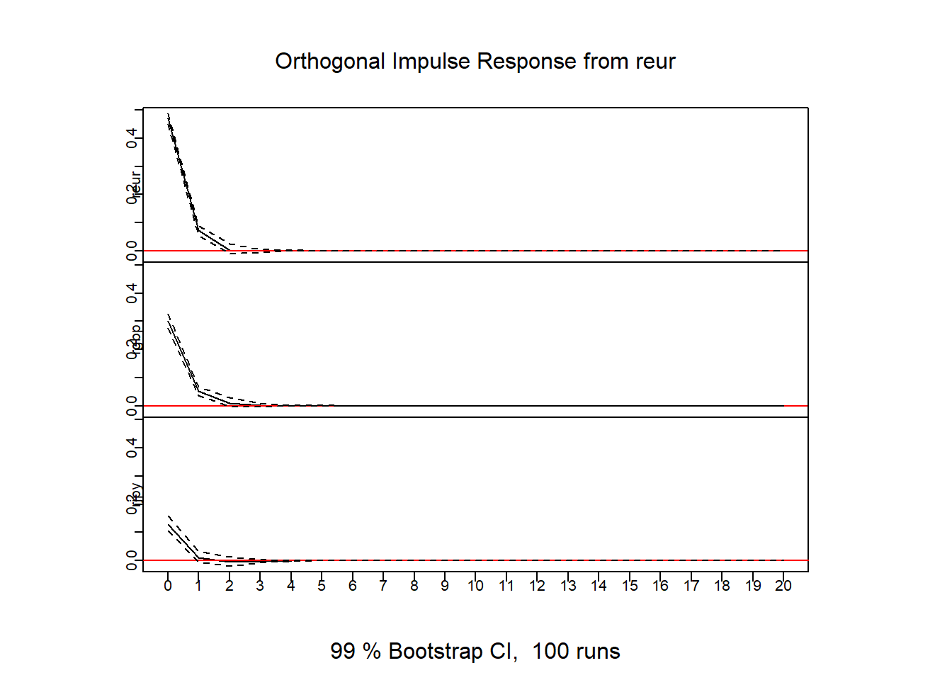
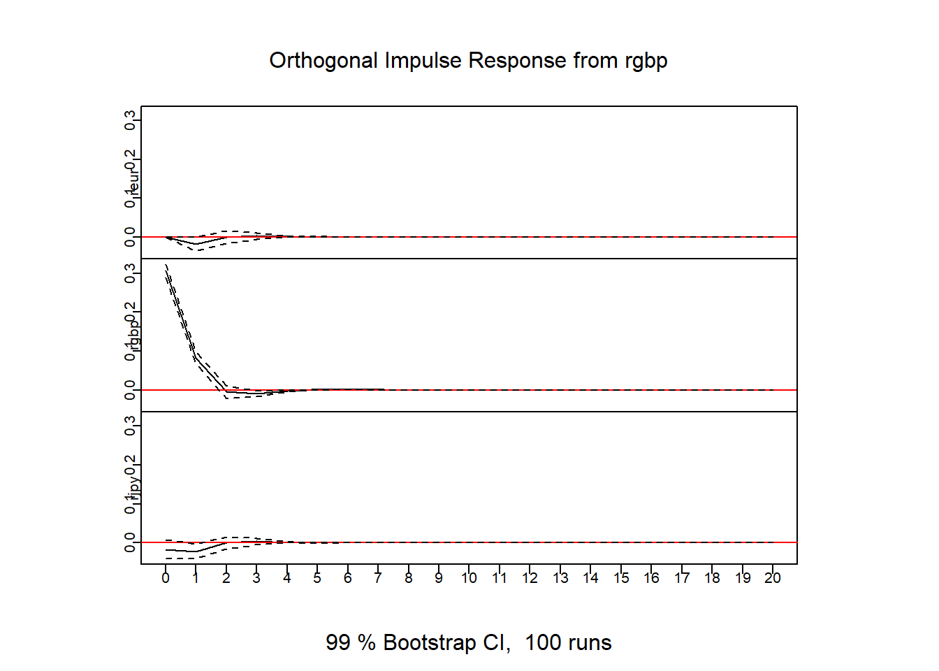
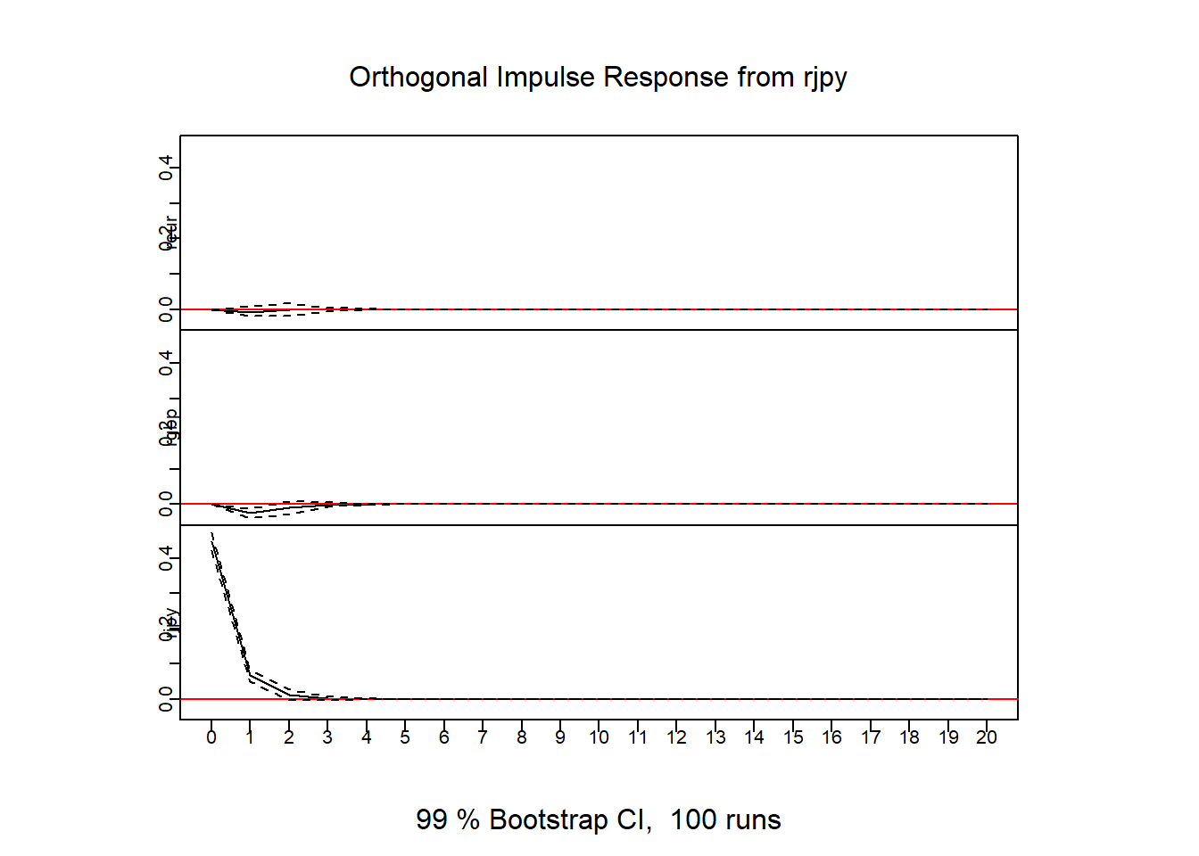
Screenshot 7.5 Combined impulse response graphs (Page 349)
par(mfcol = c(3,1), oma = c(0,0,1,0) + 0.2, mar = c(0,1,0,0) + 1, mgp = c(0, 0.2, 0))
irf.cur = irf(VAR.cur,n.ahead=20,ortho=TRUE,boot=TRUE,ci=0.99)
plot(irf.cur,col=1)
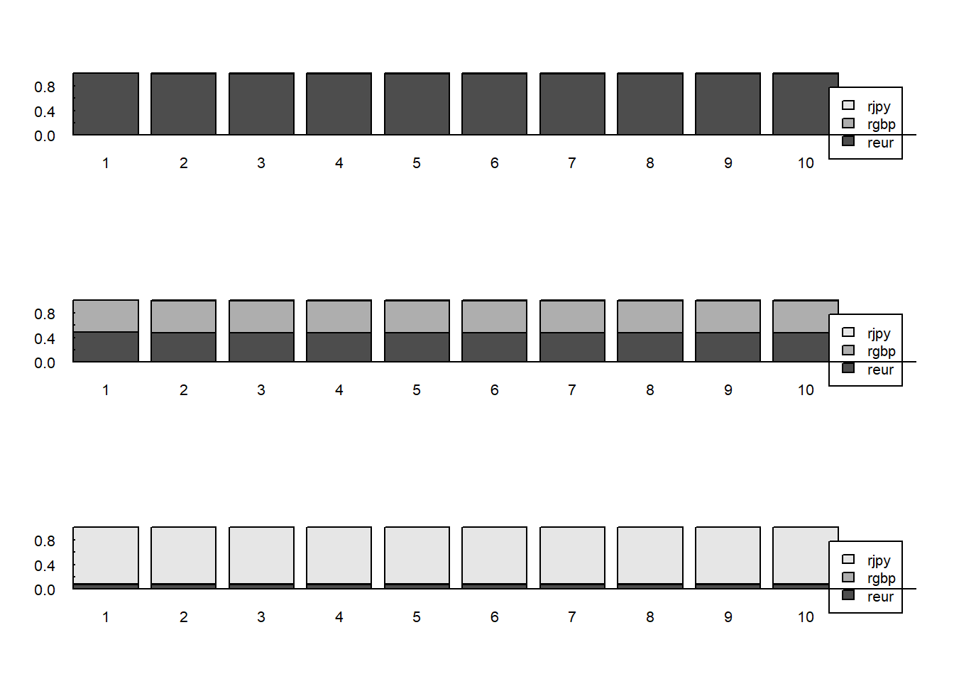
Screenshot 7.6 Variance decomposition graphs (Page 350)
fevd.cur <- fevd(VAR.cur)
fevd.cur
## $reur
##            reur        rgbp         rjpy
##  [1,] 1.0000000 0.000000000 0.0000000000
##  [2,] 0.9981178 0.001524051 0.0003581120
##  [3,] 0.9981148 0.001526281 0.0003589032
##  [4,] 0.9980823 0.001558801 0.0003589082
##  [5,] 0.9980779 0.001563074 0.0003589907
##  [6,] 0.9980779 0.001563074 0.0003590174
##  [7,] 0.9980779 0.001563127 0.0003590180
##  [8,] 0.9980778 0.001563133 0.0003590181
##  [9,] 0.9980778 0.001563133 0.0003590181
## [10,] 0.9980778 0.001563133 0.0003590181
##
## $rgbp
##            reur      rgbp        rjpy
##  [1,] 0.4895160 0.5104840 0.000000000
##  [2,] 0.4781687 0.5185439 0.003287417
##  [3,] 0.4781410 0.5181839 0.003675103
##  [4,] 0.4779089 0.5184136 0.003677557
##  [5,] 0.4778931 0.5184284 0.003678533
##  [6,] 0.4778929 0.5184284 0.003678769
##  [7,] 0.4778925 0.5184287 0.003678767
##  [8,] 0.4778925 0.5184287 0.003678769
##  [9,] 0.4778925 0.5184287 0.003678769
## [10,] 0.4778925 0.5184287 0.003678769
##
## $rjpy
##             reur        rgbp      rjpy
##  [1,] 0.07763026 0.001327719 0.9210420
##  [2,] 0.07630518 0.003773124 0.9199217
##  [3,] 0.07636047 0.003771074 0.9198685
##  [4,] 0.07636993 0.003828557 0.9198015
##  [5,] 0.07636975 0.003834408 0.9197958
##  [6,] 0.07636976 0.003834414 0.9197958
##  [7,] 0.07636976 0.003834499 0.9197957
##  [8,] 0.07636976 0.003834506 0.9197957
##  [9,] 0.07636976 0.003834506 0.9197957
## [10,] 0.07636976 0.003834506 0.9197957
plot(fevd.cur,las=1,xlab="",ylab="",main="",xaxs="i",yaxs="i",tck=.02)