CAPM Regression (Page 144)
data_capm <- read.dta("Dataset/capm.dta")
summary(lm1 <- lm(erford ~ ersandp, data = data_capm))
##
## Call:
## lm(formula = erford ~ ersandp, data = data_capm)
##
## Residuals:
##     Min      1Q  Median      3Q     Max
## -48.758  -7.248  -1.305   5.755  63.299
##
## Coefficients:
##             Estimate Std. Error t value Pr(>|t|)
## (Intercept)  -0.3199     1.0864  -0.294    0.769
## ersandp       2.0262     0.2377   8.523 2.98e-14 ***
## ---
## Signif. codes:  0 '***' 0.001 '**' 0.01 '*' 0.05 '.' 0.1 ' ' 1
##
## Residual standard error: 12.62 on 133 degrees of freedom
##   (1 observation deleted due to missingness)
## Multiple R-squared:  0.3532, Adjusted R-squared:  0.3484
## F-statistic: 72.64 on 1 and 133 DF,  p-value: 2.981e-14
Macro Data Regression and Subset Selection (Page 145)
data <- read.dta("Dataset/macro.dta")
dspread <- diff(data$BAAAAASPREAD)
dcredit <- diff(data$CONSUMERCREDIT)
dprod <- diff(data$Industrialproduction)
rmsoft <- 100 * diff(log(data$Microsoft))
rsandp <- 100 * diff(log(data$SANDP))
dmoney <- diff(data$M1MONEYSUPPLY)
inflation <- 100 * diff(log(data$CPI))
term <- data$USTB10Y - data$USTB3M
dinflation <- diff(inflation)
mustb3m <- data$USTB3M / 12
rterm <- diff(term)
ermsoft <- rmsoft - mustb3m[-1]
ersandp <- rsandp - mustb3m[-1]

data=na.omit(data)
summary(lm2 <- lm(ermsoft ~ ersandp + dprod + dcredit + dinflation + dmoney + dspread + rterm, data = data))
##
## Call:
## lm(formula = ermsoft ~ ersandp + dprod + dcredit + dinflation +
##     dmoney + dspread + rterm, data = data)
##
## Residuals:
##     Min      1Q  Median      3Q     Max
## -66.985  -3.643   1.105   6.661  26.587
##
## Coefficients:
##               Estimate Std. Error t value Pr(>|t|)
## (Intercept) -1.514e-01  9.048e-01  -0.167   0.8672
## ersandp      1.360e+00  1.566e-01   8.687   <2e-16 ***
## dprod       -1.426e+00  1.324e+00  -1.076   0.2825
## dcredit     -4.053e-05  7.640e-05  -0.530   0.5961
## dinflation   2.960e+00  2.166e+00   1.366   0.1728
## dmoney      -1.109e-02  3.518e-02  -0.315   0.7528
## dspread      5.367e+00  6.914e+00   0.776   0.4382
## rterm        4.316e+00  2.515e+00   1.716   0.0872 .
## ---
## Signif. codes:  0 '***' 0.001 '**' 0.01 '*' 0.05 '.' 0.1 ' ' 1
##
## Residual standard error: 12.66 on 316 degrees of freedom
## Multiple R-squared:  0.2068, Adjusted R-squared:  0.1892
## F-statistic: 11.77 on 7 and 316 DF,  p-value: 2.537e-13
Stepwise regression (Page 149)
#Option 1

data2 = na.omit(data)
summary(step(lm(ermsoft ~ ersandp + dprod + dcredit + dinflation + dmoney + dspread + rterm, data = data2), direction = "both"))
## Start:  AIC=1652.75
## ermsoft ~ ersandp + dprod + dcredit + dinflation + dmoney + dspread +
##     rterm
##
##              Df Sum of Sq   RSS    AIC
## - dmoney      1      15.9 50654 1650.8
## - dcredit     1      45.1 50683 1651.0
## - dspread     1      96.5 50734 1651.4
## - dprod       1     185.7 50823 1651.9
## - dinflation  1     299.2 50937 1652.7
## <none>                    50638 1652.8
## - rterm       1     471.8 51109 1653.8
## - ersandp     1   12091.6 62729 1720.1
##
## Step:  AIC=1650.85
## ermsoft ~ ersandp + dprod + dcredit + dinflation + dspread +
##     rterm
##
##              Df Sum of Sq   RSS    AIC
## - dcredit     1      45.4 50699 1649.2
## - dspread     1      85.2 50739 1649.4
## - dprod       1     174.9 50828 1650.0
## - dinflation  1     311.1 50965 1650.8
## <none>                    50654 1650.8
## - rterm       1     492.3 51146 1652.0
## + dmoney      1      15.9 50638 1652.8
## - ersandp     1   12079.7 62733 1718.2
##
## Step:  AIC=1649.15
## ermsoft ~ ersandp + dprod + dinflation + dspread + rterm
##
##              Df Sum of Sq   RSS    AIC
## - dspread     1      79.5 50778 1647.7
## - dprod       1     208.1 50907 1648.5
## - dinflation  1     295.3 50994 1649.0
## <none>                    50699 1649.2
## - rterm       1     487.8 51187 1650.2
## + dcredit     1      45.4 50654 1650.8
## + dmoney      1      16.2 50683 1651.0
## - ersandp     1   12036.0 62735 1716.2
##
## Step:  AIC=1647.65
## ermsoft ~ ersandp + dprod + dinflation + rterm
##
##              Df Sum of Sq   RSS    AIC
## - dprod       1     234.7 51013 1647.2
## - dinflation  1     240.3 51019 1647.2
## <none>                    50778 1647.7
## - rterm       1     481.6 51260 1648.7
## + dspread     1      79.5 50699 1649.2
## + dcredit     1      39.7 50739 1649.4
## + dmoney      1       4.9 50774 1649.6
## - ersandp     1   12089.8 62868 1714.8
##
## Step:  AIC=1647.15
## ermsoft ~ ersandp + dinflation + rterm
##
##              Df Sum of Sq   RSS    AIC
## - dinflation  1     308.0 51321 1647.1
## <none>                    51013 1647.2
## + dprod       1     234.7 50778 1647.7
## - rterm       1     488.2 51501 1648.2
## + dspread     1     106.0 50907 1648.5
## + dcredit     1      72.5 50941 1648.7
## + dmoney      1       0.0 51013 1649.2
## - ersandp     1   12186.6 63200 1714.5
##
## Step:  AIC=1647.1
## ermsoft ~ ersandp + rterm
##
##              Df Sum of Sq   RSS    AIC
## <none>                    51321 1647.1
## + dinflation  1     308.0 51013 1647.2
## + dprod       1     302.4 51019 1647.2
## - rterm       1     448.3 51769 1647.9
## + dcredit     1      59.3 51262 1648.7
## + dspread     1      35.9 51285 1648.9
## + dmoney      1       3.2 51318 1649.1
## - ersandp     1   12167.6 63489 1714.0
##
## Call:
## lm(formula = ermsoft ~ ersandp + rterm, data = data2)
##
## Residuals:
##     Min      1Q  Median      3Q     Max
## -66.806  -3.909   1.080   6.253  29.637
##
## Coefficients:
##             Estimate Std. Error t value Pr(>|t|)
## (Intercept)  -0.6858     0.7037  -0.975    0.331
## ersandp       1.3372     0.1533   8.724   <2e-16 ***
## rterm         4.1815     2.4970   1.675    0.095 .
## ---
## Signif. codes:  0 '***' 0.001 '**' 0.01 '*' 0.05 '.' 0.1 ' ' 1
##
## Residual standard error: 12.64 on 321 degrees of freedom
## Multiple R-squared:  0.1961, Adjusted R-squared:  0.1911
## F-statistic: 39.15 on 2 and 321 DF,  p-value: 6.094e-16
# Option 2
library(olsrr)
# Fit the initial model
model <- lm(ermsoft ~ ersandp + dprod + dcredit + dinflation + dmoney + dspread + rterm, data = data2)
# Run stepwise regression with p-value thresholds
ols_step_both_p(model, prem = 0.2, add = 0.2)
##
##
##                                Stepwise Summary
## -----------------------------------------------------------------------------
## Step    Variable         AIC         SBC         SBIC        R2       Adj. R2
## -----------------------------------------------------------------------------
##  0      Base Model     2635.292    2642.853    1715.376    0.00000    0.00000
##  1      ersandp (+)    2569.387    2580.729    1649.926    0.18908    0.18656
##  2      rterm (+)      2568.569    2583.692    1649.166    0.19610    0.19109
## -----------------------------------------------------------------------------
##
## Final Model Output
## ------------------
##
##                           Model Summary
## -----------------------------------------------------------------
## R                       0.443       RMSE                  12.586
## R-Squared               0.196       MSE                  158.398
## Adj. R-Squared          0.191       Coef. Var          -4059.606
## Pred R-Squared          0.183       AIC                 2568.569
## MAE                     7.528       SBC                 2583.692
## -----------------------------------------------------------------
##  RMSE: Root Mean Square Error
##  MSE: Mean Square Error
##  MAE: Mean Absolute Error
##  AIC: Akaike Information Criteria
##  SBC: Schwarz Bayesian Criteria
##
##                                 ANOVA
## ----------------------------------------------------------------------
##                  Sum of
##                 Squares         DF    Mean Square      F         Sig.
## ----------------------------------------------------------------------
## Regression    12519.039          2       6259.520    39.152    0.0000
## Residual      51321.051        321        159.879
## Total         63840.090        323
## ----------------------------------------------------------------------
##
##                                   Parameter Estimates
## ---------------------------------------------------------------------------------------
##       model      Beta    Std. Error    Std. Beta      t        Sig      lower    upper
## ---------------------------------------------------------------------------------------
## (Intercept)    -0.686         0.704                 -0.975    0.331    -2.070    0.699
##     ersandp     1.337         0.153        0.437     8.724    0.000     1.036    1.639
##       rterm     4.181         2.497        0.084     1.675    0.095    -0.731    9.094
## ---------------------------------------------------------------------------------------
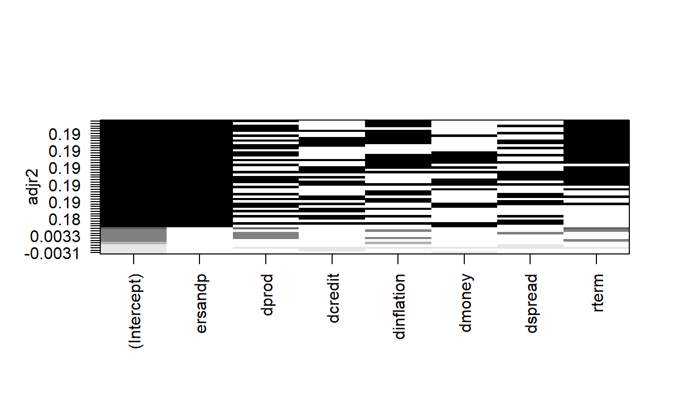
Model Selection Plot (Page 149)
leaps <- regsubsets(ermsoft ~ ersandp + dprod + dcredit + dinflation + dmoney + dspread + rterm, data = data2, nbest = 10)
plot(leaps, scale = "adjr2")
Quantile Regression (Page 165)
data_capm <- read.dta("Dataset/capm.dta")
BETA <- sapply(seq(0.1, 0.9, by = 0.1), function(tau) {
  coef(rq(erford ~ ersandp, data = data_capm, tau = tau))
})
summary(BETA)
##        V1                V2                V3                V4                V5
##  Min.   :-12.425   Min.   :-8.2948   Min.   :-5.5927   Min.   :-4.2950   Min.   :-1.62658
##  1st Qu.: -8.719   1st Qu.:-5.7596   1st Qu.:-3.7946   1st Qu.:-2.8035   1st Qu.:-0.80512
##  Median : -5.013   Median :-3.2245   Median :-1.9965   Median :-1.3121   Median : 0.01635
##  Mean   : -5.013   Mean   :-3.2245   Mean   :-1.9965   Mean   :-1.3121   Mean   : 0.01635
##  3rd Qu.: -1.307   3rd Qu.:-0.6893   3rd Qu.:-0.1983   3rd Qu.: 0.1794   3rd Qu.: 0.83781
##  Max.   :  2.399   Max.   : 1.8458   Max.   : 1.5998   Max.   : 1.6709   Max.   : 1.65927
##        V6              V7              V8              V9
##  Min.   :1.039   Min.   :1.652   Min.   :1.971   Min.   : 1.615
##  1st Qu.:1.222   1st Qu.:1.924   1st Qu.:3.257   1st Qu.: 4.821
##  Median :1.404   Median :2.196   Median :4.543   Median : 8.026
##  Mean   :1.404   Mean   :2.196   Mean   :4.543   Mean   : 8.026
##  3rd Qu.:1.586   3rd Qu.:2.467   3rd Qu.:5.829   3rd Qu.:11.232
##  Max.   :1.768   Max.   :2.739   Max.   :7.116   Max.   :14.438
plot(seq(0.1, 0.9, 0.1), BETA[1, ], type = "o", las = 1, pch = 20,
     xlab = "Quantiles", ylab = "Coefficients", main = "Quantile Regression Coefficients", tck = 0.02)
points(seq(0.1, 0.9, 0.1), BETA[2, ], type = "o", col = "steelblue4", pch = 20)
legend("topright", legend = c("Intercept", "Slope"), col = c("black", "steelblue4"), pch = 20, box.col = "white")

Eigenvalue Analysis (Page 175)
data <- read.dta("Dataset/macro.dta")
interest_rates <- data[, c("USTB3M", "USTB6M", "USTB1Y", "USTB3Y", "USTB5Y", "USTB10Y")]

cor_matrix <- cor(interest_rates)
eigen_results <- eigen(cor_matrix)

eigen_results$vectors
##            [,1]       [,2]       [,3]       [,4]        [,5]        [,6]
## [1,] -0.4066368 -0.4482369  0.5146117 -0.4606699 -0.31374158  0.24135964
## [2,] -0.4089605 -0.3963105  0.1013554  0.1983160  0.49874699 -0.61427894
## [3,] -0.4121447 -0.2712975 -0.3164404  0.5987738 -0.05905395  0.54257020
## [4,] -0.4143717  0.1175832 -0.5612330 -0.2183381 -0.53942127 -0.40104989
## [5,] -0.4098192  0.3646077 -0.2212300 -0.4656201  0.57610655  0.31853709
## [6,] -0.3973398  0.6493495  0.5107271  0.3541896 -0.16265369 -0.08784986
## [1] 5.7917388755 0.1973202793 0.0080995259 0.0022349759 0.0004044343 0.0002019091
diff(eigen_results$values)
## [1] -5.5944185961 -0.1892207534 -0.0058645500 -0.0018305416 -0.0002025251
variance_proportions <- eigen_results$values / sum(eigen_results$values)
variance_proportions
## [1] 9.652898e-01 3.288671e-02 1.349921e-03 3.724960e-04 6.740571e-05 3.365152e-05
cumulative_variance <- cumsum(variance_proportions)
cumulative_variance
## [1] 0.9652898 0.9981765 0.9995264 0.9998989 0.9999663 1.0000000